Choreographing the spins inside Diamond

Products & Services

Resources

News & Events

Company

Book a demo

All blog posts

Choreographing the spins inside Diamond

In this blog post, we will describe open loop optimal control of various gates on a diamond based quantum processor using the Qruise toolset.

1. Diamond quantum processors
2. Quantum information processing with a diamond quantum processor
3. Diamond quantum processor with Qruise toolset
4. Optimal control of single Qubit gates
5. Optimal control of two qubit gates
6. Optimal control of three qubit gates
References

1 Diamond quantum processors

1.1 The constituents

Diamond quantum processors are promising platform for quantum technology applications. Their ability to work at ambient conditions, requirement of relatively simple control electronics, and biocompatibility makes them attractive candidates for quantum information processing [1] and quantum sensing [2].

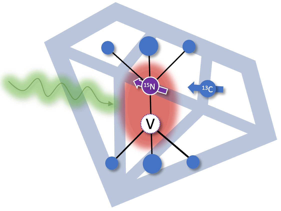
A diamond quantum processor consists of an nitrogen vacancy (NV) center and multiple nuclear spins which are coupled to it via hyperfine interactions. The NV centers are formed in diamond crystal by knocking off a few carbon atoms via high energy irradiation followed by high temperature annealing. The coupled nuclear spins include intrinsic nuclear spin of the nitrogen atom ( ${}^{15}\text{N}$ and ${}^{14}\text{N}$ ) and surrounding isotopic impurities ( ${}^{13}\text{C}$ ). The nuclear spins act as the physical qubits on this processor and the NV centre is used as a quantum bus to initialize, readout, and perform gate operations on coupled nuclear spins [3].

1.2 Physical properties

All the important physical properties of a diamond processor can be explained using following energy level structure

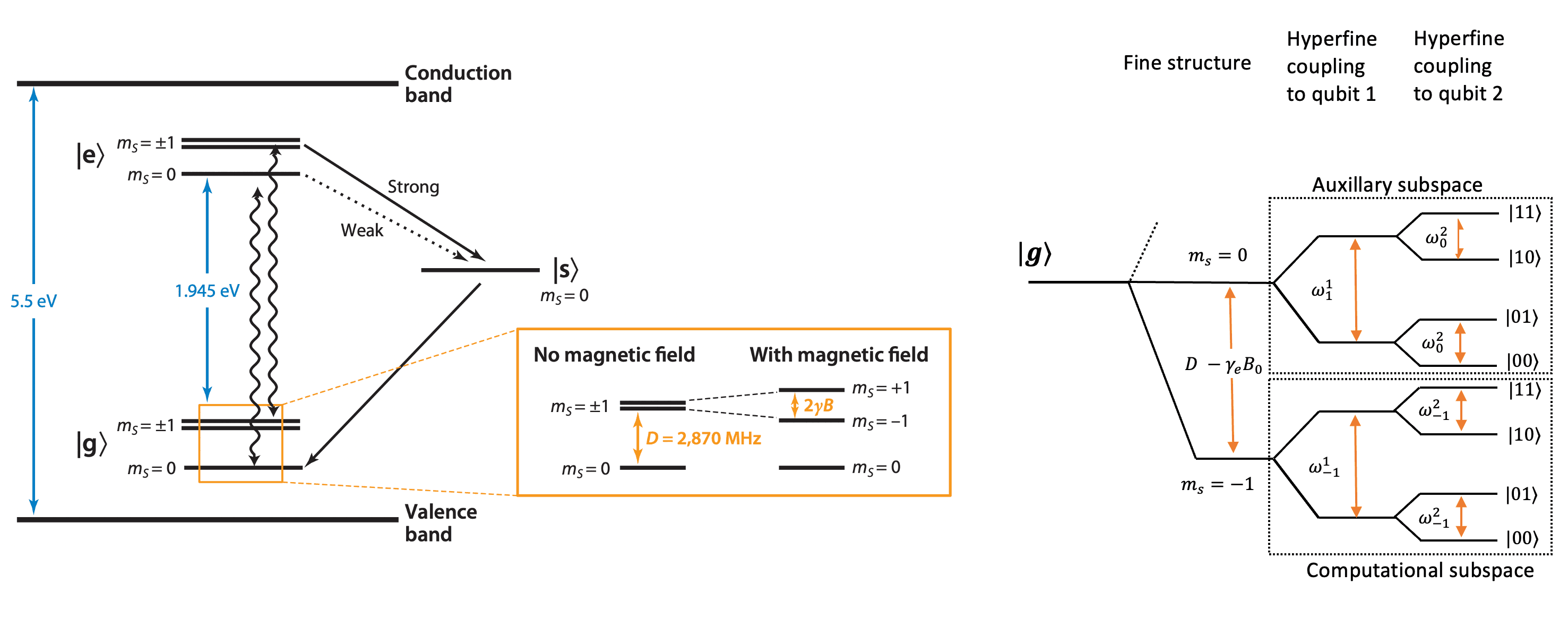
Fig 1. Energy level structure of a NV center coupled to two nuclear spins which act as physical qubits. The figure is adapted from Ref [3] and Ref [4].

1.2.1 Electronic level structure

The NV center is a one of the fluorescent lattice defects inside diamond and all its basic photophysics can be described by three electronic levels, a ground level $|g\rangle$ , a excited level $|e\rangle$ and a metastable level $|s\rangle$ .

1.2.2 Spin level structure

The ground and excited state are spin triplet (total spin $S = 1$ ) and further split into 3 sublevels ( $m_s = 0, \pm 1$ ). The $m_s = \pm 1$ levels are degenerate, and the energy gap between them and $m_s = 0$ level is $D = 2.87$ GHz in ground state and $D = 1.42$ GHz in excited state. The parameter $D$ is called zero field splitting. Due to hyperfine interactions with nuclear spins, the spin levels are further split depending on the number of nuclear spins and coupling strength.

The degeneracy between $m_s = \pm 1$ levels can be lifted by applying a magnetic field causing them to move in opposite directions. This feature is often used to approximate the NV center as a two level system by only considering $m_s = 0$ and $m_s = -1$ levels.

1.2.3 Optical properties

The initialization and read out of NV center happens by optical means and metastable state $|s\rangle$ plays a pivotal role in it. When the NV center is pumped with radiation of appropriate wavelength (typically 532nm), the $m_s = 0$ state mainly decays via radiative transition whereas the $m_s = \pm 1$ states level has a higher probability to decay through the metastable state. This spin-selective decay mechanism causes a contrast between $m_s = 0$ and $m_s = \pm 1$ levels (typically 30%) which lasts for the lifetime of metastable state ( $\approx 300$ ns) and is used to readout the state of NV center. To initialize NV center into $m_s = 0$ state, laser excitation for longer duration ( $\approx 1-2\mu$ s) is used since metastable state eventually decays to repopulate $m_s = 0$ states.

1.3 Hamiltonian model

In this blog post, we will consider a diamond quantum processor made up of three spins , an NV center and two nuclear spins ( ${}^{13}\text{C}$ and a ${}^{15}\text{N}$ or ${}^{14}\text{N}$ ) coupled to it. The full Hamiltonian of the system can be written as

$\begin{aligned} H = D \left(S*z^2-\frac{2}{3}\right) + \gamma_e B_0 S_z + \gamma_e B_1^e(t) S_x + \sum_i \vec{S} \cdot \textbf{A}\_i \cdot \vec{I_i} + Q_i \left(I*{iz}^2-\frac{2}{3}\right) + \gamma*i B_0 I*{iz} + \gamma*i B*{1}^n(t) I\_{ix} \end{aligned}$

with

$S_z / S_x$ = Spin operators of NV electron spin

$\gamma_e$ = Gyromagnetic ratio of NV electron spin

$D$ = zero-field splitting

$B_0$ = applied magnetic field

$\textbf{A}$ = Hyperfine coupling tensor

$Q_i$ = Quadrupole tensor of the $i^{\text{th}}$ nuclei (nonzero for ${}^{14}\text{N}$ )

$I_{i,z} / I_{i,x}$ = Spin operators of the $i^{\text{th}}$ nuclei

$\gamma_{i}$ = Gyromagnetic ratio of $i^{\text{th}}$ nuclei

$B_{1}^e$ = Control field applied on electron spin

$B_{1}^n$ = Control field applied on the nuclei

Typically, only two out of three spin subspaces are required for computation, so we ignore $m_s = 1$ subspace because it requires higher MW frequencies which are usually difficult to generate. The single qubit gates are carried out in computational space, i.e., $m_s = -1$ subspace, whereas multi qubit gates utilize auxiliary, i.e., $m_s = 0$ subspace as well.

The Hamiltonians is further simplified [3] by applying (i) secular approximation because a very strong field is applied along z-axis (ii) alignment approximation where only nuclei with hyperfine fields nearly aligned with the NV axis are chosen.

For single qubit gates on nuclei

$H_{\text{single}} = \sum_i - \omega_i I_{iz} - \gamma_i I_{ix} B_{1}^n(t) \qquad \qquad (1)$

For multi qubit gates

$H*{\text{multi}} = \frac{\Delta}{2} \sigma_z+\frac{\Omega_e}{2} B*{1}^e(t) \sigma*x + \sum_i (\alpha_i + \beta_i \sigma_z) I*{iz} + \gamma*{i} B*{1}^n(t) I\_{ix} \qquad \qquad (2)$

with

$\sigma_x$ = $|0\rangle\langle -1| + |-1\rangle\langle 0|$

$\Delta = D - \gamma_e B_0$

$\Omega = \sqrt{2}\gamma_e$

$\alpha_i = -\frac{\gamma_i B_0}{2} - \frac{\omega_i}{2}$ , where $\omega_i = \sqrt{{[A_{i,zz} + \gamma_i B_0}]^2 + A_{i,xz}^2 + A_{i,yz}^2}$ is the transition frequency, respectively, of the $i^{\text{th}}$ nuclei

$\beta_i = -\frac{\gamma_i B_0}{2} + \frac{\omega_i}{2}$

2. Quantum information processing with a diamond quantum processor

The key requirements for a universal quantum processor are initialization, readout and gate operations on qubits. On a diamond based processor, these steps require high fidelity gates both on NV electron spin and nuclear spins as described in the following sections.

2.1 Initialization

Initialization of the nuclear spin qubits occurs via following steps alternating among nuclear spins (repeated until desired state is achieved) [5]:

Polarization transfer
- (i) Initialize NV electron spin in $|0\rangle$ state
- (ii) SWAP the state of NV electron spin with nuclei. The SWAP operation is realized by two controlled gates
  - (a) Two qubit gate which is a $\pi$ gate on NV electron spin conditioned on target nuclear spin realised using microwave (MW) pulse
  - (b) Two qubit gate which is a $\pi$ gate on target nuclear spin conditioned on NV electron spin realised using radio frequency pulse (RF) pulse

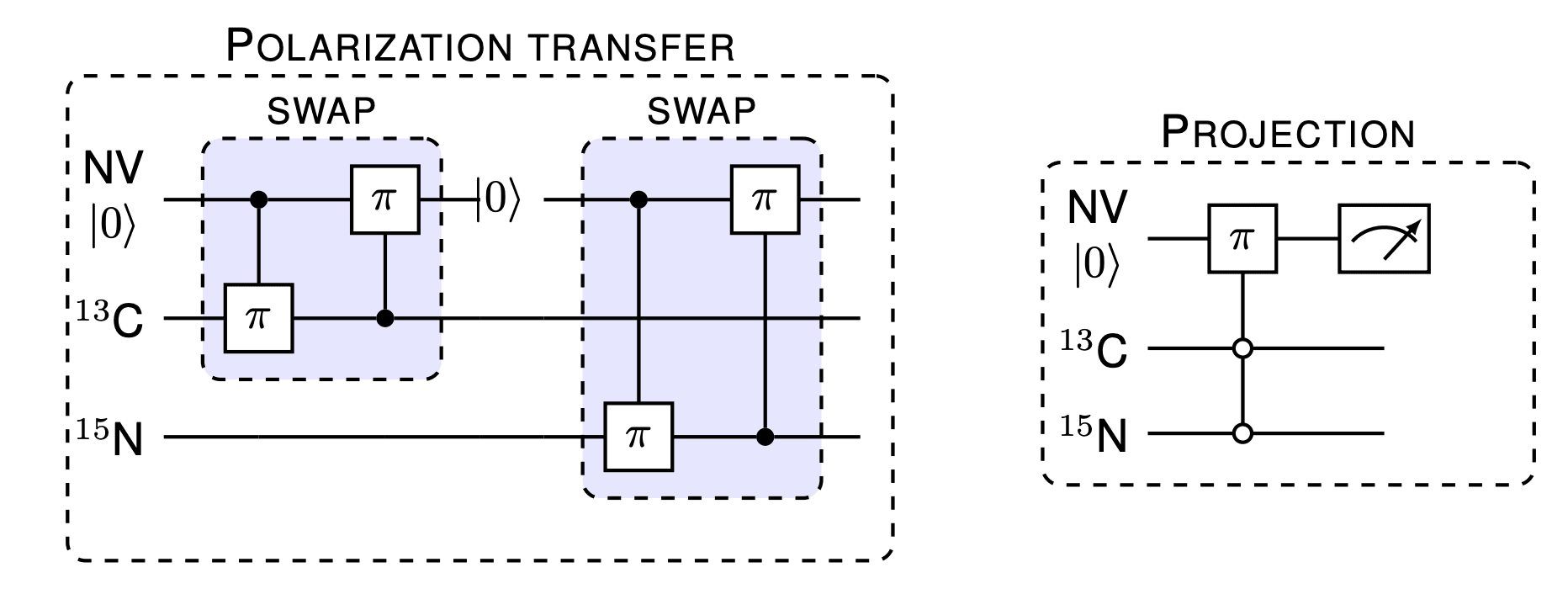
After sufficient polarization transfer, a projective measurement of nuclear register is performed to further increase initialization probability

Projection
- (i) Initialize NV electron spin in $|0\rangle$ state
- (ii) Apply a multi qubit gate which is a $\pi$ gate (MW pulse) on NV electron spin conditioned on desired state of nuclear spin register

2.2 Gate operations:

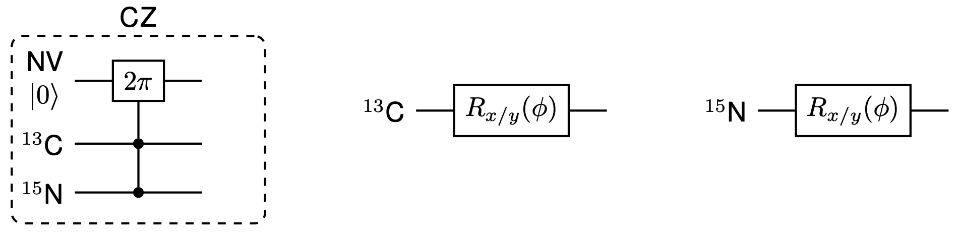
Single-qubit gate operations on this processor are $R_x(\phi)$ and $R_y(\phi)$ gates realised using RF pulses. Other single-qubit gates can be constructed from combinations of these rotations. These operations are performed by addressing the distinct resonances of the nuclear spins in the computational subspace.

The intrinsic properties of the NV-nuclear spins system allows direct application of a $CZ$ gate via MW pulses on the nuclear spin register [5]. The $CZ$ gate is achieved by performing a selective $2\pi$ pulse conditional on the nuclear spin register being in the $|11\rangle$ state. The $CZ$ gate can be combined with single-qubit gates to realise any other two-qubit gate.

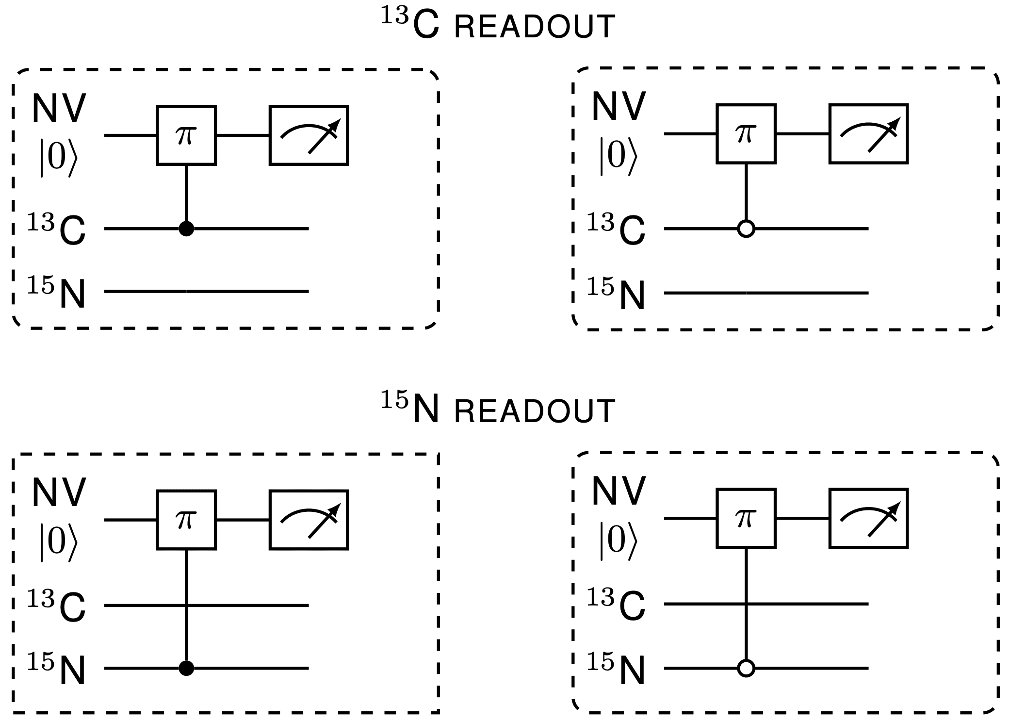
2.3 Readout:

The repetitive readout technique is also employed to read out each nuclear spin qubit at the end of a computation [6]. This involves many repetitions of

(i) Initialize NV electron spin in $|0\rangle$ state
(ii) Apply two qubit gate which is a $\pi$ gate on NV electron spin conditioned on target nuclear spin (alternate between $|0\rangle$ and $|1\rangle$ states of nuclear spin) realised using microwave (MW) pulse
(iii) Read out the electron spin state

3. Diamond quantum processor with Qruise toolset

We first start with single qubit nuclear gates which are carried out in computational subspace with Hamiltonian in Eq. (1) and we go to an interaction frame defined by $\mathcal{\tau} = e^{-i t \sum_i \omega I_{iz} }$ , where $\omega$ is the frequency of applied drive .

We assume that control field is of the form $B_{1}^n(t) = E(t) \cos(\omega t + \phi)$ , then after rotating wave approximation, in the interaction frame nuclear spin Hamiltonian transforms to

$H_\text{single} = \mathcal{\tau} H_{m_S = -1} \mathcal{\tau}^{-1} -i \mathcal{\tau} \frac{d}{dt} \mathcal{\tau}^{-1} = -\sum_i \left[\Delta \omega_i I_{iz} + \gamma_i \frac{E(t)}{2} (I_{ix} \cos{\phi} + I_{iy} \sin{\phi})\right]$

where $\Delta\omega_i = \omega_i - \omega$ is the offset of the drive from the transition frequency of the $i^{\mathrm{th}}$ nuclear spin.

In the following, the Hamiltonian in the interaction frame is implemented and we will perform a $(\pi/2)_x$ pulse on ${}^{13}\text{C}$ .

We start by importing the modules from Qruise toolset that we will use for the optimization

Click to view the module imports

# Main Qruise toolset imports

from qruise.toolset.objects import Quantity
from qruise.toolset.model import Model
from qruise.toolset.generator.generator import SimpleGenerator
from qruise.toolset.parametermap import ParameterMap
from qruise.toolset.experiment import Experiment
from qruise.toolset.signal import pulse, gates

# Imports for spin Hamiltonian

from qruise.toolset.libraries.nvcentres.components import Spin, DriveSpin
from qruise.toolset.libraries.nvcentres.hamiltonians import x_drive_spin, y_drive_spin
from qruise.toolset.libraries.nvcentres.hamiltonians import spin_coupling_zz

# Optimal Control imports

from qruise.toolset.optimizers.optimalcontrol import OptimalControl
import qruise.toolset.libraries.fidelities as fidelities
import qruise.toolset.libraries.algorithms as algorithms
from qruise.toolset.optimizers.loggers import PlotLineChart

# Pulse shape

from qruise.toolset.libraries.envelopes import  pwl_shape_sampled_times

# Other imports

import copy
import numpy as np
import tensorflow as tf

3.1 Parameters of the system

Now we define the parameters of the system, including the magnetic field strength, the gyromagnetic ratio, and the transition frequencies of the nuclear spins.

B_0 = 6200.0  # in Gauss
Gauss_to_Tesla = 0.0001
B_0 = B_0 * Gauss_to_Tesla

A_zz_C13 = 2.281e6  # Hz
A_xz_C13 = 0.24e6  # Hz
A_yz_C13 = 0.24e6  # Hz
A_zz_N15 = 3.03e6  # Hz
A_xz_N15 = 0.0  # Hz
A_yz_N15 = 0.0  # Hz


gyromag_ratio_N15_val = -4.316e6  # Hz/T
gyromag_ratio_C13_val = 10.7084e6  # Hz/T

omega_C13 = np.sqrt(
    (A_zz_C13 + gyromag_ratio_C13_val * B_0) ** 2 + A_xz_C13**2 + A_yz_C13**2
)
omega_N15 = np.sqrt(
    (A_zz_N15 + gyromag_ratio_N15_val * B_0) ** 2 + A_xz_N15**2 + A_yz_N15**2
)

freq_C13_val = omega_C13
freq_N15_val = omega_N15

offset_C13_val  = omega_C13-freq_C13_val # Offset on C13 is zero because we want to a gate on it
offset_N15_val  = omega_N15-freq_C13_val # Offset on N15 is -3.99 MHz approximately

3.2 Defining the Spin

In Qruise toolset, the spins are defined by Spin class where we need to specify the Hilbert space dimension, in this case 2 for every spin unless ${}^{14}\text{N}$ is also included which has 3 levels instead. Along with that we need to specify offset or detuning of the drive from the transition frequency of the spin in terms of Qruise Quantity (take a look at our introductory blog: Learn to drive (qubits) with Qruise to learn more about it )

# NV
nv = Spin(
    name="NV",
    hilbert_dim=2,
    desc="NV spin",
    params={
        "offset": Quantity(value=0.0, min_val=-0.5e3, max_val=+0.5e3, unit=" Hz 2pi")
    },
)
# C13
c13 = Spin(
    name="C13",
    hilbert_dim=2,
    desc="Carbon-13 spin",
    params={
        "offset": Quantity(
            value=offset_C13_val,
            min_val=offset_C13_val - 0.5e3,
            max_val=offset_C13_val + 0.5e3,
            unit=" Hz 2pi",
        )
    },
)

# N15
n15 = Spin(
    name="N15",
    hilbert_dim=2,
    desc="Nitrogen-15 spin",
    params={
        "offset": Quantity(
            value=offset_N15_val,
            min_val=offset_N15_val - 0.5e3,
            max_val=offset_N15_val + 0.5e3,
            unit=" Hz 2pi",
        )
    },
)

3.3 Driving the Spin

For single qubit gates, we need to drive ${}^{13}\text{C}$ and ${}^{15}\text{N}$ to stir the dynamics. The drives of spins in the Qruise toolset are defined using the DriveSpin class where we can specify the direction of the drive. Here, we set up drives along both $x$ and $y$ axis

drive_c13_x = DriveSpin(
    name="drive_c13_x",
    desc="Drive along x axis c13",
    comment="",
    connected=["C13"],
    hamiltonian_func=x_drive_spin,
)
drive_c13_y = DriveSpin(
    name="drive_c13_y",
    desc="Drive along y axis on c13",
    comment="",
    connected=["C13"],
    hamiltonian_func=y_drive_spin,
)
drive_n15_x = DriveSpin(
    name="drive_n15_x",
    desc="Drive along x axis on n15",
    comment="",
    connected=["N15"],
    hamiltonian_func=x_drive_spin,
)
drive_n15_y = DriveSpin(
    name="drive_n15_y",
    desc="Drive along x axis on n15",
    comment="",
    connected=["N15"],
    hamiltonian_func=y_drive_spin,
)

3.4 Making the Model

Next we connect the components (defined above) together using the Qruise Model class. Here we can set subsystems for the model (spins in our case), drives on them, coupling between them, basis for Hamiltonian (if dressed is required), and Lindblad dynamics (dephasing or dissipation)

model = Model(
    subsystems=[nv, c13, n15],
    couplings=[drive_c13_x, drive_c13_y, drive_n15_x, drive_n15_y],
    tasks=[],
    dressed=False,
    lindbladian=False,
    use_FR=True,
)

3.5 Generator

A Generator is essential for specifying the coupling between the spins and the drives. Qruise toolset provides a lot of flexibility regarding the control electronics and various devices such as Local Oscillator (LO), Arbitrary Waveform Generator (AWG), Digital to Analog converter (DAC) and a Mixer using the Generator object. Here we use SimpleGenerator which assumes all the devices to be ideal.

v2Hz = 1e6
awg_res = 1e9
generator = SimpleGenerator(
    V_to_Hz=Quantity(value=v2Hz, min_val=0.9 * v2Hz, max_val=1.1 * v2Hz, unit="Hz/V"),
    awg_res=awg_res,
)

To know more about signal generation with Qruise, please take a look at our introductory blog Learn to drive (qubits) with Qruise

Pulse shapes

Now we will choose the shape of the envelope applied to the spin which will be optimized later. First we set the Rabi frequency and duration of the operations:

Rabi_freq  = 2*np.pi*2.5e6
ampl_val_hz = Rabi_freq/2/np.pi # the amplitude applied to spin in Hz
ampl_val_c13 = ampl_val_hz/v2Hz
ampl_val_n15 = ampl_val_hz/v2Hz
t_final = 1.458e-6  # Gate duration

Again, Qruise toolset provides a lot of flexibility on choosing the pulse envelope shape through pulse class, for example, square, gaussian, Fourier basis to name a few. Here we use a piecewise linear envelope where we divide the total time of pulse on a specified number of bins and use linear interpolation between the bins. Later, we will feed this envelope to the optimizer which will carry out a Gradient based optimization to find optimal shape. This pulse shape has been previously utilized successfully optimize gates on a diamond quantum processor ( [5], [7], [8], [9]).

n_bins = 100
grape_pulse = pulse.Envelope(
   name="GRAPE envelope_c13",
   params={
       "t_sampled": Quantity(value=np.linspace(0, t_final, n_bins)),
       "inphase": Quantity(
           value=ampl_val_c13 * np.random.rand(n_bins),
           min_val=0,
           max_val=2 * ampl_val_c13,
           unit="V",
       ),
       "t_final": Quantity(
           value=t_final, min_val=0.9 * t_final, max_val=1.1 * t_final, unit="s"
       ),
   },
   shape=pwl_shape_sampled_times,
)

Carrier wave

Each drive component has to have a carrier associated with it. Since these simulations are carried out in the interaction frame of the drive, we can set the Carrier frequency to zero for both the qubits.

carr_1 = pulse.Carrier(
  name="carrier",
  desc="Frequency of the local oscillator",
  params={
      "freq": Quantity(
          value=0.0, min_val=-freq_C13_val, max_val=freq_C13_val, unit="Hz 2pi"
      ),
      "framechange": Quantity(
          value=0.0, min_val=-np.pi, max_val=3 * np.pi, unit="rad"
      ),
  },
)

lo_freq_q2 = 0.0
carr_2 = copy.deepcopy(carr_1)
carr_2.params["freq"].set_value(lo_freq_q2)

3.6 Defining the Instruction

Now, we specify what specific gate operation we intend to apply upon our spins using the pulse. Here, as an example, we want to instruct our pulse to perform the $(\pi/2)_x$ gate on ${}^{13}\text{C}$ .

rx90p_c13 = gates.Instruction(
   name="rx90p",
   targets=[1],
   t_start=0.0,
   t_end=t_final,
   channels=["drive_c13_x", "drive_n15_x"],
)

rx90p_c13.add_component(grape_pulse, "drive_c13_x")
rx90p_c13.add_component(copy.deepcopy(carr_1), "drive_c13_x")
rx90p_c13.add_component(grape_pulse, "drive_n15_x")
rx90p_c13.add_component(copy.deepcopy(carr_2), "drive_n15_x")

3.7 Setting the parameter map

We now combine the model, generator, and instructions into what we call the ParameterMap

parameter_map = ParameterMap(instructions=[rx90p_c13], model=model, generator=generator)

3.8 Defining the experiment

After defining the parameter map, we are ready to instantiate a experiment using Experiment class

sim_res =2e9
exp = Experiment(pmap=parameter_map, sim_res=sim_res,prop_method="pwc")

3.9 Simulating the dynamics

The actual numerical simulation is done by calling exp.compute_propagators(). This is the most resource intensive part as it involves solving the equations of motion for the system.

unitaries = exp.compute_propagators()

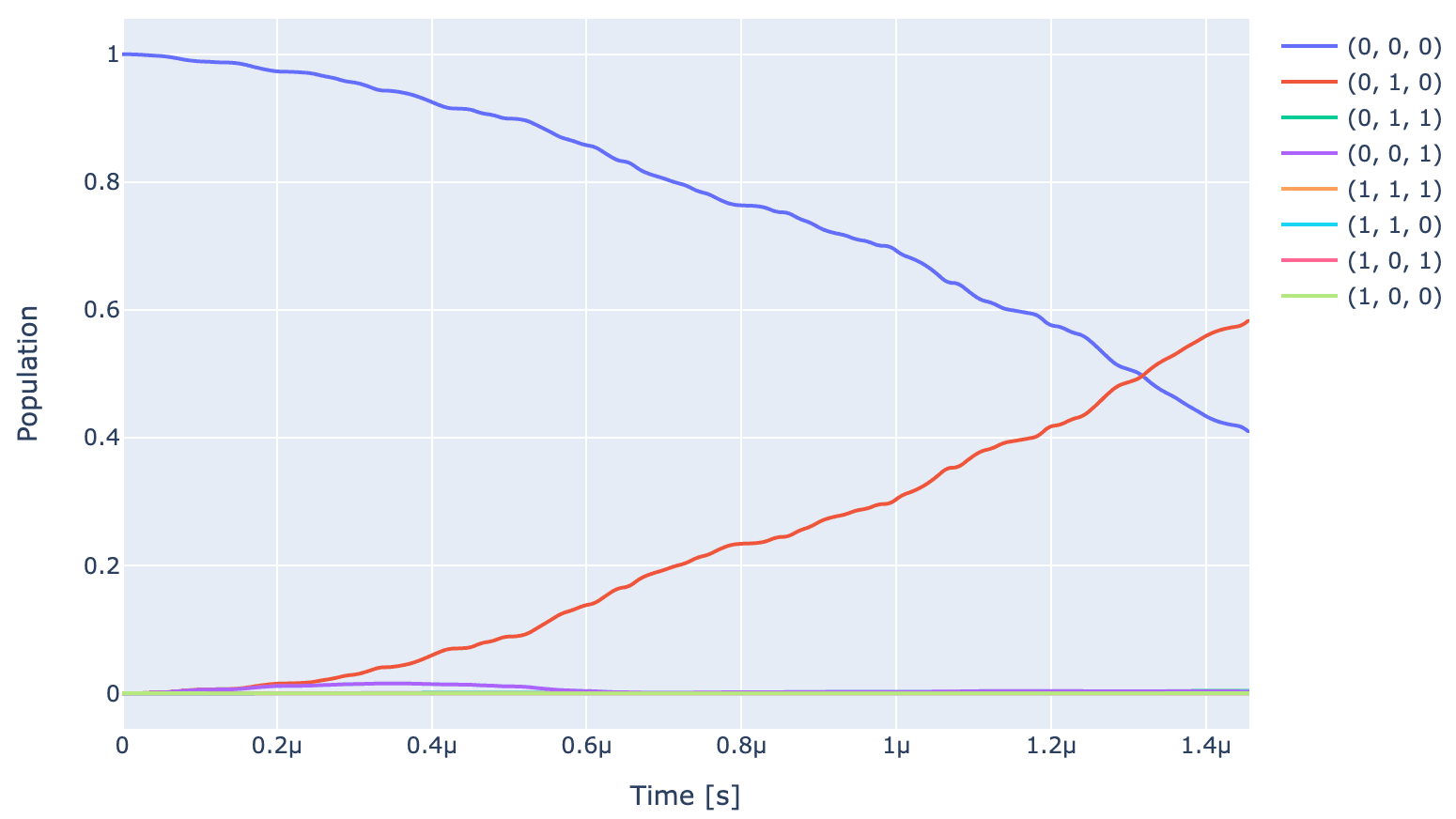
Next we define a initial state and visualize the population dynamics

psi_init = [[0] * 8]
psi_init[0][0] = 1
initial_state = tf.transpose(tf.constant(psi_init, dtype=tf.complex128))
Sequence = [rx90p_c13.get_key()]
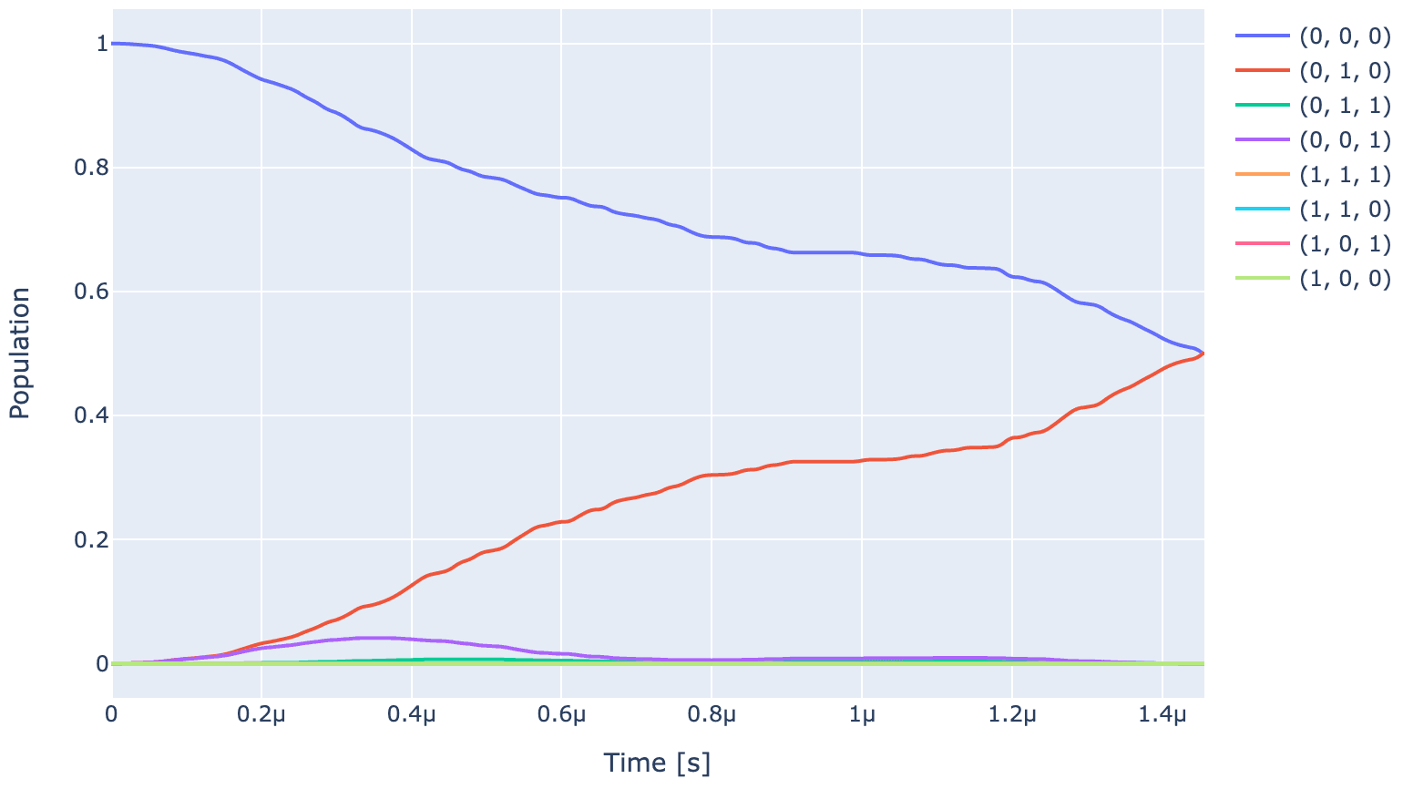
exp.draw_dynamics(Sequence, initial_state)

In ideal case, $(\pi/2)_x$ pulse should cause (i) population in $|000\rangle$ state to get divided equally between $|000\rangle$ and $|010\rangle$ , and (ii) populations in other states should go to zero. However, since the gate is not optimized, the above two conditions occur at slightly different time points.

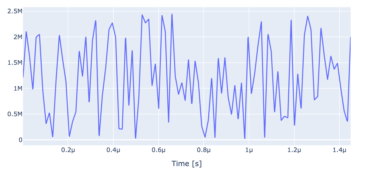
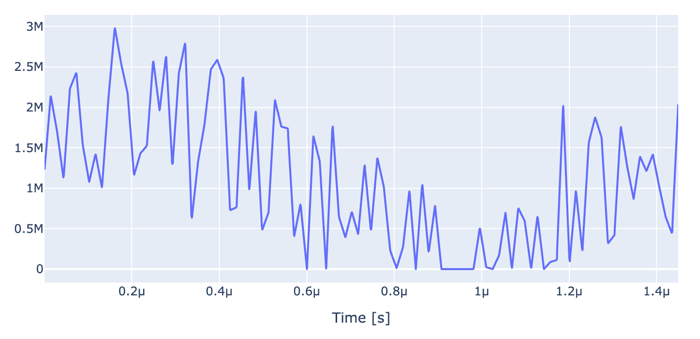
We can also look at the pulse envelope which causes the above dynamics. The $y$ axis is in the unit of Hz. It is a envelope which is randomly varies between minimum and maximum value of allowed amplitude

generator.draw(opt_gate, awg_res, centered=True)

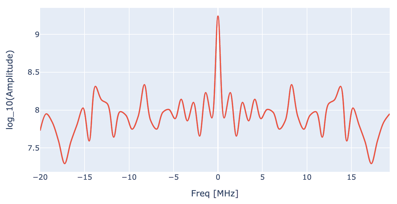
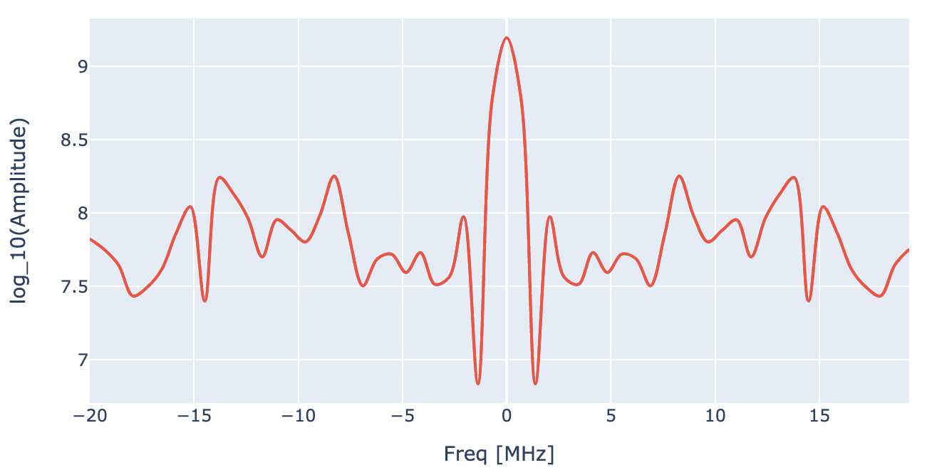
Fourier transform of the pulse can be plotted using following call for further insights into pulse

generator.draw_spectrum(opt_gate, awg_res, draw_spectrograms=False,freq_scale=1e6, freq_range=[-20e6,20e6])

4 Optimal control of single qubit gates

4.1 Setting the optimal parameter map

First we set the pulse parameters to be optimized

drive_opt_map = [
    [(opt_gate.get_key(), "drive_c13_x", "GRAPE envelope_c13", "inphase")],
    [(opt_gate.get_key(), "drive_c13_x", "GRAPE envelope_c13", "t_final")],
    ]

    parameter_map.set_opt_map(drive_opt_map)

4.2 Setting up and running the optimizer

Using OptimalControl class, we can set the cost function, optimization algorithm and monitor the progress of optimization using the logger. Here, we use unitary infidelity overlap function $f = 1- |\text{Tr}[U_{\text{ideal}} U_{\text{opt}}^\dagger]|^2$ as cost function and gradient based L- BFGS as optimization algorithm

opt = OptimalControl(dir_path=log_dir,
                    fid_func=fidelities.unitary_infid_set,
                    fid_subspace=["NV", "C13", "N15"],
                    pmap=parameter_map,
                    algorithm=algorithms.lbfgs,
                    options={"maxfun": 100},
                    run_name="better_Y90_C13",
                    logger=[PlotLineChart()]
)

Starting optimization: The logger shows infidelity at various optimization steps.

opt.set_exp(exp)
opt.optimize_controls()

4.3 Analysing the optimal solutions

After the optimization is over, we can check the best fidelity using following call

print(f"Gate Fidelity: {(1 - opt.current_best_goal) * 100} %")
Gate Fidelity: 99.99999970303573 %

After optimization, we compute the propagators again with optimized control parameters and view the optimized dynamics

exp.compute_propagators()
exp.draw_dynamics(Sequence, initial_state)

As expected, affter application of optimal control population of $|000\rangle$ state gets divided equally between $|000\rangle$ and $|010\rangle$ and populations in rest of the states go to zero.

Finally, let's plot at the optimized pulse and its Fourier transform which corresponds to optimal high fidelity gate

generator.draw(opt_gate, awg_res)

generator.draw_spectrum(opt_gate, awg_res, draw_spectrograms=False,freq_scale=1e6, freq_range=[-20e6,20e6])

5 Optimal control of two qubit gates

Now we turn our focus onto optimization of multi-qubit gates using Qruise toolset. The implementation of mullti-qubit gates is governed by Eq (2). The steps involved to set up the Hamiltonian model and optimal control are exactly same to what we describe in case of single qubit gates. We start by defining the value of Hamiltonian parameters :

D = 2.87e9  # Hz # zero field splitting
gyromag_ratio_NV_val = 28.024e9  # Hz/T
B_0 = 1000.0  # in Gauss
Gauss_to_Tesla = 0.0001
B_0 = B_0 * Gauss_to_Tesla
Delta = D - gyromag_ratio_NV_val * B_0

A_zz_C13 = 2.281e6 #Hz
A_xz_C13 = 0.24e6  #Hz
A_yz_C13 = 0.24e6 #Hz
A_zz_N15 = 3.03e6 # Hz
A_xz_N15 = 0.0 #Hz
A_yz_N15 = 0.0 #Hz


gyromag_ratio_N15_val = -4.316e6  # Hz/T
gyromag_ratio_C13_val = 10.7084e6  # Hz/T

omega_C13 = np.sqrt(
    (A_zz_C13 + gyromag_ratio_C13_val * B_0) ** 2 + A_xz_C13**2 + A_yz_C13**2
)  # MHz
omega_N15 = np.sqrt(
    (A_zz_N15 + gyromag_ratio_N15_val * B_0) ** 2 + A_xz_N15**2 + A_yz_N15**2
)  # MHz

alpha_C13 = -0.5*(gyromag_ratio_C13_val * B_0 + omega_C13)
alpha_N15 = -0.5*(gyromag_ratio_N15_val * B_0 + omega_N15)
beta_C13 =  -0.5*(gyromag_ratio_C13_val * B_0 - omega_C13)
beta_N15 =  -0.5*(gyromag_ratio_N15_val * B_0 - omega_N15)

Now we define the spins

# NV
nv = Spin(
    name="NV",
    hilbert_dim=2,
    desc="NV spin",
    params={
        "offset": Quantity(
            value=Delta, min_val=Delta - 0.5e3, max_val=Delta + 0.5e3, unit="Hz 2pi"
        ),
    },
)

# C13
c13 = Spin(
    name="C13",
    hilbert_dim=2,
    desc="Carbon-13 spin",
    params={
        "offset": Quantity(
            value=alpha_C13,
            min_val=alpha_C13 - 0.5e3,
            max_val=alpha_C13 + 0.5e3,
            unit="Hz 2pi",
        ),
    },
)

# N15
n15 = Spin(
    name="N15",
    hilbert_dim=2,
    desc="Nitrogen-15 spin",
    params={
        "offset": Quantity(
            value=alpha_N15,
            min_val=alpha_N15 - 0.5e3,
            max_val=alpha_N15 + 0.5e3,
            unit="Hz 2pi",
        ),
    },
)

and coupling between the spins using Coupling class where species connected via coupling, coupling strength and form of the coupling can be specified


# Coupling between NV and nuclear spins
nv_c13 = Coupling(
    name="NV-C13",
    desc="coupling",
    comment="Coupling NV to C13",
    connected=["NV", "C13"],
    strength=Quantity(
        value=beta_C13, min_val=0.9 * beta_C13, max_val=1.1 * beta_C13, unit="Hz 2pi"
    ),
    hamiltonian_func=spin_coupling_zz,
)


nv_n15 = Coupling(
    name="NV-N15",
    desc="coupling",
    comment="Coupling NV to N15",
    connected=["NV", "N15"],
    strength=Quantity(
        value=beta_N15, min_val=0.9 * beta_N15, max_val=1.1 * beta_N15, unit="Hz 2pi"
    ),
    hamiltonian_func=spin_coupling_zz,
)

Next we set up drive on the spins


# Drives on the spins
drive_nv = DriveSpin(
    name="drive_nv",
    desc="Drive along x axis for NV spin",
    comment="",
    connected=["NV"],
    hamiltonian_func=x_drive_spin,
)

drive_c13 = DriveSpin(
    name="drive_c13",
    desc="Drive along x axis for C13 spin",
    comment="",
    connected=["C13"],
    hamiltonian_func=x_drive_spin,
)

drive_n15 = DriveSpin(
    name="drive_n15",
    desc="Drive along x axis for N15 spin",
    comment="",
    connected=["N15"],
    hamiltonian_func=x_drive_spin,
)

Connecting the components together and making the model. We again set up a closed system model in computational basis

model = Model(
    subsystems=[nv, c13, n15],
    couplings=[nv_c13, nv_n15, drive_nv, drive_c13, drive_n15],
    tasks=[],
    dressed=False,
    lindbladian=False,
    use_FR=True,
)

Setting up the "ideal" control stack with SimpleGenerator

v2Hz = 1e6
awg_res = 1e9
generator = SimpleGenerator(
   V_to_Hz=Quantity(value=v2Hz, min_val=0.9 * v2Hz, max_val=1.1 * v2Hz, unit="Hz/V"),
   awg_res=awg_res,
)

Now we define carrier frequencies for the spins. The two qubit controlled gates are realized using MW or RF pulses. These pulse are realized by drives whose carrier frequency set on the targeted spin. Since, there are multiple transitions corresponding to each spin, we set the carrier frequency at the mean frequency of these transitions.

To calculate the transition frequencies, we get the time-independent hamiltonian from our model

H_drift = model._matrix_provider.drift_hamiltonian_components
H_TI = (
   H_drift["NV"]
   + H_drift["C13"]
   + H_drift["N15"]
   + H_drift["NV-C13"]
   + H_drift["NV-N15"]
)

Since, the time-independent Hamiltonian is already diagonal, we simply calculate the transition frequencies as follows

eigvals = np.linalg.eig(H_TI)[0]

transtion_freqs_nv = [
   eigvals[0] - eigvals[4], # 000 -> 100
   eigvals[1] - eigvals[5], # 001 -> 101
   eigvals[2] - eigvals[6], # 010 -> 110
   eigvals[3] - eigvals[7], # 011 -> 111
]

transtion_freqs_c13 = [
   eigvals[0] - eigvals[2], # 000 -> 010
   eigvals[1] - eigvals[3], # 001 -> 011
   eigvals[4] - eigvals[6], # 100 -> 110
   eigvals[5] - eigvals[7], # 101 -> 111
]

transtion_freqs_n15 = [
   eigvals[0] - eigvals[1], # 000 -> 001
   eigvals[2] - eigvals[3], # 010 -> 011
   eigvals[4] - eigvals[5], # 100 -> 101
   eigvals[6] - eigvals[7], # 110 -> 111
]

Now we set the carrier wave frequencies of various spin to be equal to their respective mean transition frequency

lo_freq_nv = np.real(np.mean(transtion_freqs_nv))/2/np.pi
lo_freq_c13 = np.real(np.mean(transtion_freqs_c13))/2/np.pi
lo_freq_n15 = np.real(np.mean(transtion_freqs_n15))/2/np.pi

carr_nv = pulse.Carrier(
    name="carrier",
    desc="Frequency of the local oscillator",
    params={
        "freq": Quantity(
            value=lo_freq_nv,
            min_val=lo_freq_nv - 0.5e3,
            max_val=lo_freq_nv + 0.5e3,
            unit="Hz 2pi",
        ),
        "framechange": Quantity(
            value=0.0, min_val=-np.pi, max_val=3 * np.pi, unit="rad"
        ),
    },
)

carr_c13 = pulse.Carrier(
    name="carrier",
    desc="Frequency of the local oscillator",
    params={
        "freq": Quantity(
            value=lo_freq_c13,
            min_val=lo_freq_c13 - 0.5e3,
            max_val=lo_freq_c13 + 0.5e3,
            unit="Hz 2pi",
        ),
        "framechange": Quantity(
            value=0.0, min_val=-np.pi, max_val=3 * np.pi, unit="rad"
        ),
    },
)

carr_n15 = pulse.Carrier(
    name="carrier",
    desc="Frequency of the local oscillator",
    params={
        "freq": Quantity(
            value=lo_freq_n15,
            min_val=lo_freq_n15 - 0.5e3,
            max_val=lo_freq_n15 + 0.5e3,
            unit="Hz 2pi",
        ),
        "framechange": Quantity(
            value=0.0, min_val=-np.pi, max_val=3 * np.pi, unit="rad"
        ),
    },
)

Here, we will demonstrate optimal control of a controlled gate which amounts to $(\pi)_x$ RF pulse of ${}^{15}\text{N}$ spin conditioned on $|1\rangle$ state of NV spin. Accordingly, we set the Rabi frequency and gate duration for ${}^{15}\text{N}$ spin

Rabi_freq_n15 = 2 * np.pi * 10e6
ampl_val_hz_n15 = Rabi_freq_n15 / 2 / np.pi
ampl_val_n15 = ampl_val_hz_n15 / v2Hz
t_final_n15 = 2.1e-6

Next, we define a piecewise linear envelope for the RF pulse for that will implement the gate

n_bins = 500
grape_pulse_n15 = pulse.Envelope(
    name="GRAPE envelope_n15",
    params={
        "t_sampled": Quantity(value=np.linspace(0, t_final_n15, n_bins)),
        "inphase": Quantity(
            value=ampl_val_n15 * np.ones(n_bins),
            min_val=0,
            max_val=5 * ampl_val_n15,
            unit="V",
        ),
        "t_final": Quantity(
            value=t_final_n15,
            min_val=0.9 * t_final_n15,
            max_val=1.1 * t_final_n15,
            unit="s",
        ),
    },
    shape=pwl_shape_sampled_times,
)

Now let's define the desired controlled gate in terms of instructions. The ideal gate for the instruction is typically defined in a interaction frame where time-independent of Hamiltonian is absent. However, since we have implemented the lab-frame Hamiltonian above, we convert the definition of ideal gate to lab frame via transformation: $U_{\text{int}} = e^{-i H_{\text{TI}} t}$

Uint_n15 = expm(-1j*H_TI.numpy()*t_final_n15)

C_nv_X_n15_int = np.array(
    [
        [1, 0, 0, 0, 0, 0, 0, 0],
        [0, 1, 0, 0, 0, 0, 0, 0],
        [0, 0, 1, 0, 0, 0, 0, 0],
        [0, 0, 0, 1, 0, 0, 0, 0],
        [0, 0, 0, 0, 0, -1j, 0, 0],
        [0, 0, 0, 0, -1j, 0, 0, 0],
        [0, 0, 0, 0, 0, 0, 0, -1j],
        [0, 0, 0, 0, 0, 0, -1j, 0],
    ],
    dtype=np.complex128,
)

C_nv_X_n15_lab = Uint_n15 @ C_nv_X_n15_int

C_nv_X_n15 = gates.Instruction(
    name="C_nv_X_n15",
    targets=[0, 1, 2],
    t_start=0.0,
    t_end=t_final_n15,
    channels=["drive_n15"],
    ideal=C_nv_X_n15_lab,
)
C_nv_X_n15.add_component(grape_pulse_n15, "drive_n15")
C_nv_X_n15.add_component(carr_n15, "drive_n15")

Combining the model, generator, and instructions into the ParameterMap

opt_gate = C_nv_X_n15
parameter_map = ParameterMap(instructions=[opt_gate], model=model, generator=generator)

Initiating the experiment and compute the propagators to simulate the dynamics


sim_res = 2e9  # Resolution for numerical simulation
exp = Experiment(pmap=parameter_map, sim_res=sim_res, prop_method="pwc")
unitaries = exp.compute_propagators()

Next, we define initial state and sequence which is simply the gate we want to implement

psi_init = [[0] * 8]
psi_init[0][4] = 1
psi_init[0][6] = 1

initial_state = tf.transpose(tf.constant(psi_init, dtype=tf.complex128))
Sequence = [opt_gate.get_key()]

Now let's plot the simulated dynamics under unoptimized pulse (shown in the next plot)


exp.draw_dynamics(Sequence, initial_state)

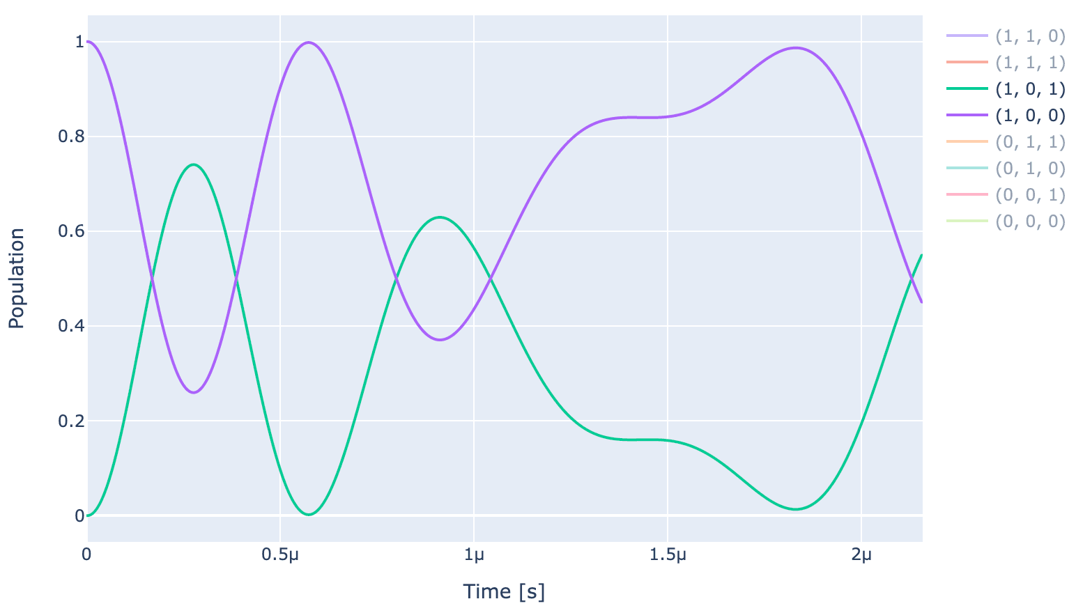
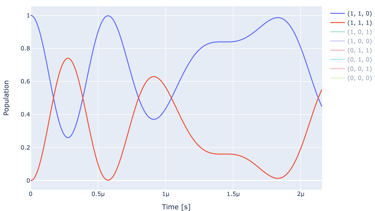
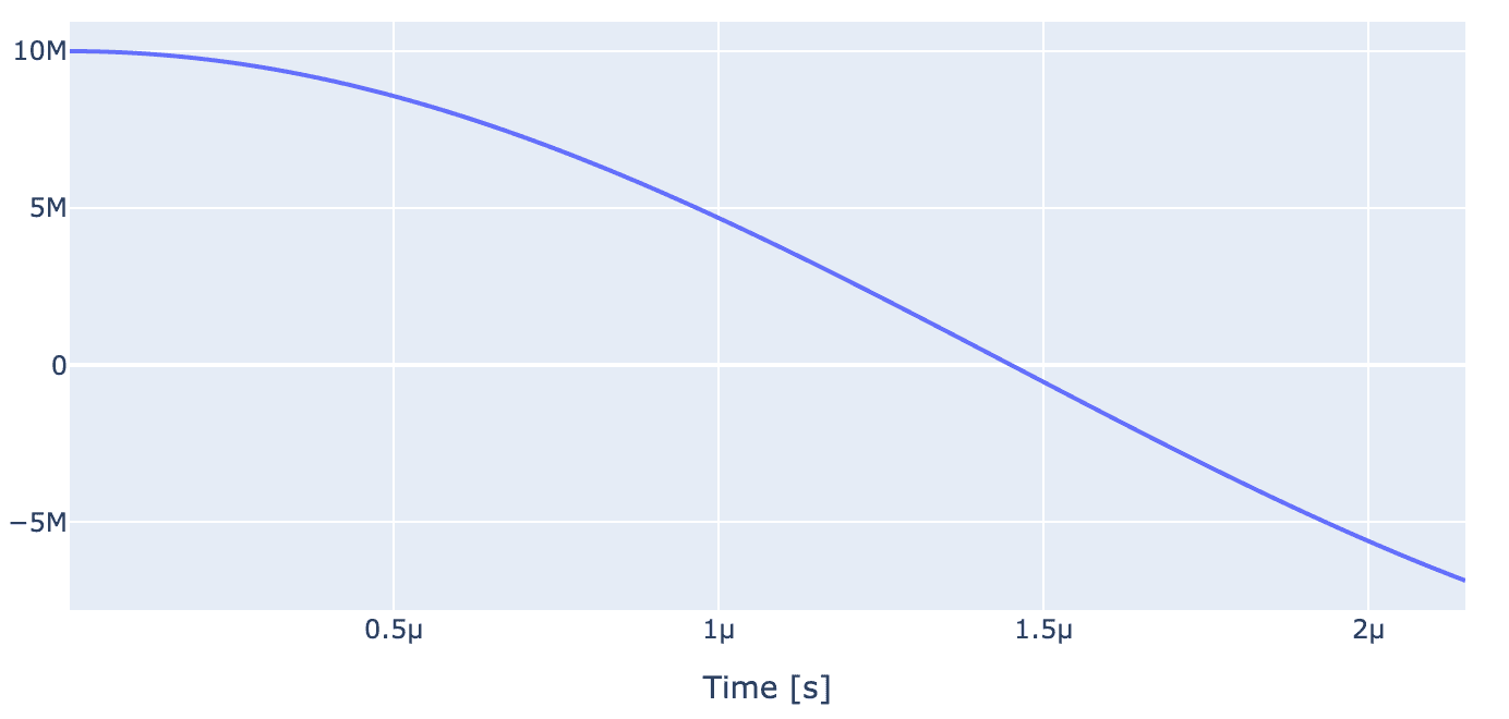
For an optimal gate, $|100\rangle \leftrightarrow |101\rangle$ and $|110\rangle \leftrightarrow |111\rangle$ , and rest of the states will return back to their initial states. As visible from the dynamics above, the unoptimized pulse (shown below) is far from achieving that


generator.draw(opt_gate, sim_res, centered=True)

Now we set up optimal control to improve gate fidelity. Starting with setting up the parameters to be optimized


 drive_opt_map = [
        [(opt_gate.get_key(), "drive_n15", "GRAPE envelope_n15", "inphase")],
        [(opt_gate.get_key(), "drive_n15", "GRAPE envelope_n15", "t_final")],
    ]

  parameter_map.set_opt_map(drive_opt_map)

We feed the parameter map into OptimalControl object along with setting the cost function, optimization algorithm and Logger


import os
import tempfile

# Create a temporary directory to store logfiles, modify as needed
log_dir = os.path.join(tempfile.TemporaryDirectory().name, "qruiselogs")

opt = OptimalControl(
  dir_path=log_dir,
  fid_func=fidelities.unitary_infid_set,
  fid_subspace=["NV", "C13", "N15"],
  pmap=parameter_map,
  algorithm=algorithms.lbfgs,
  options={"maxfun": 300},
  run_name="better_control_gate",
  logger=[PlotLineChart()],
)

Starting the optimisation

opt.set_exp(exp)
opt.optimize_controls()

After a few itirations, the optimzer achives high fidelity

print(f"Gate Fidelity: {(1 - opt.current_best_goal) * 100} %")
Gate Fidelity: 99.9999933694210 %

Recalculating the propagators and drawing the optimized dynamics


unitaries = exp.compute_propagators()
exp.draw_dynamics(Sequence, initial_state)

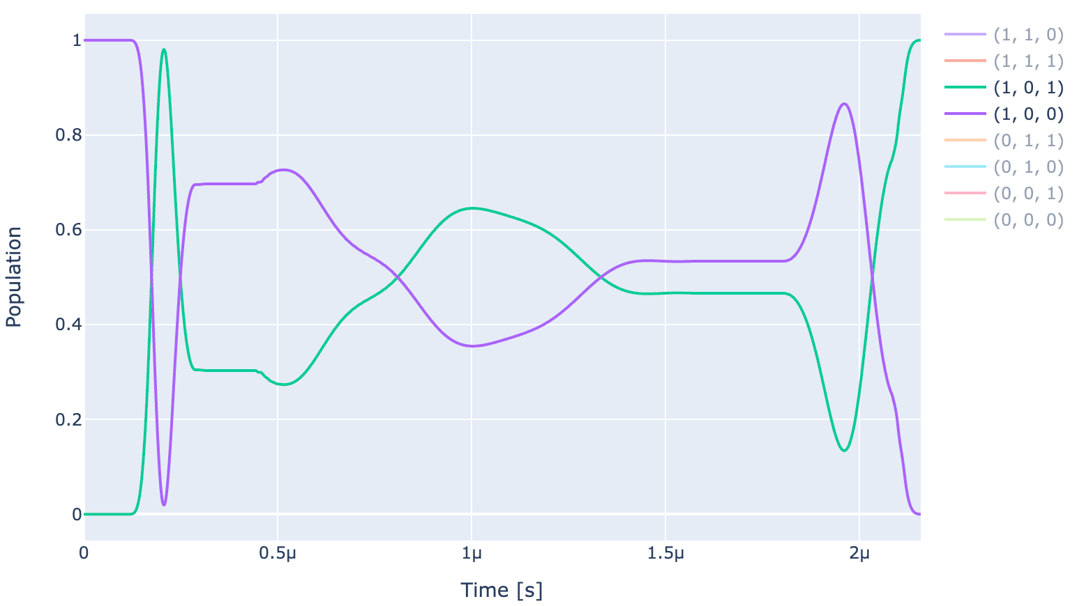
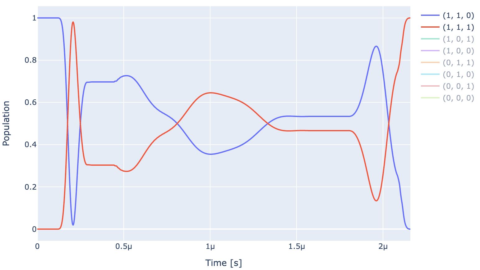
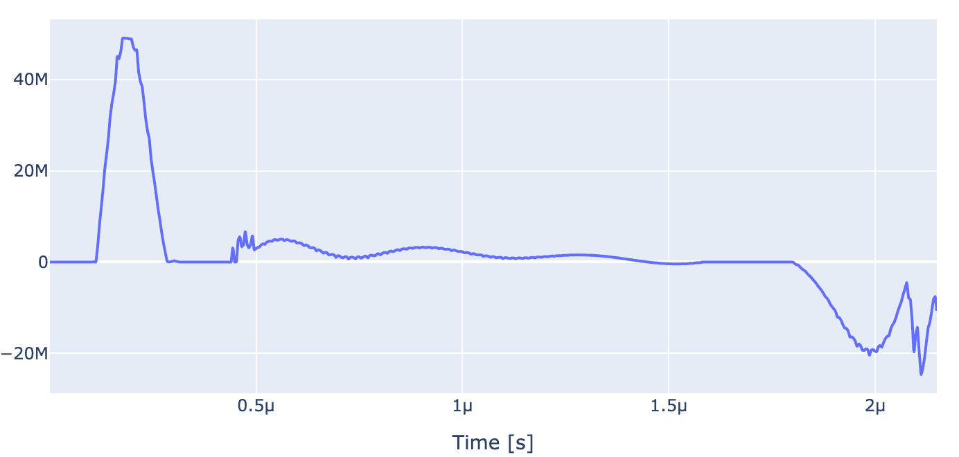
As can be observed from the above plot, the optimizer is able to produce a pulse (shown below) which produces the expected ideal behaviour, i.e., $|100\rangle \leftrightarrow |101\rangle$ and $|110\rangle \leftrightarrow |111\rangle$ , and rest of the states return back to their initial states.

generator.draw(opt_gate, awg_res)

6 Optimal control of three qubit gates

Now we move on to three qubit gates. The whole setup for optimal control of three qubit gates is exactly similar to two qubit gates. We will only change definition of the carrier frequency, target gate, initial state and pulse parameters.

We will implement a controlled gate which will flip the NV spin conditioned on $|11\rangle$ state of nuclei. Since it is a transition selective gate, we set the carrier frequency to be frequency of this transition

lo_freq = np.real(transtion_freqs_nv[3]) / 2 / np.pi

carr_nv = pulse.Carrier(
    name="carrier",
    desc="Frequency of the local oscillator",
    params={
        "freq": Quantity(
            value=lo_freq_nv,
            min_val=lo_freq_nv - 0.5e3,
            max_val=lo_freq_nv + 0.5e3,
            unit="Hz 2pi",
        ),
        "framechange": Quantity(
            value=0.0, min_val=-np.pi, max_val=3 * np.pi, unit="rad"
        ),
    },
)

Next we set the Rabi frequency for NV and gate duration

Rabi_freq_nv  = 2*np.pi*10e6
ampl_val_hz_nv = Rabi_freq_nv/2/np.pi # the amplitude applied to spin in Hz
ampl_val_nv = np.sqrt(2)* ampl_val_hz_nv/ v2Hz
t_final_nv = 3.07e-6

Setting the piecewise linear pulse to drive NV spins

n_bins = 600
grape_pulse_nv = pulse.Envelope(
   name="GRAPE envelope_nv",
   params={
       "t_sampled": Quantity(value=np.linspace(0, t_final_nv, n_bins)),
       "inphase": Quantity(
           value=ampl_val_nv * np.ones(n_bins), min_val=0, max_val=6 * ampl_val_nv, unit="V"
       ),
       "t_final": Quantity(
           value=t_final_nv, min_val=0.9 * t_final_nv, max_val=1.1 * t_final_nv, unit="s"
       ),
   },
   shape=pwl_shape_sampled_times,
)

Setting the instruction as the desired gate

Uint = expm(-1j*H_TI.numpy()*t_final_nv)

C_11_2pi_e_ideal_int = np.array(
    [
        [1, 0, 0, 0, 0, 0, 0, 0],
        [0, 1, 0, 0, 0, 0, 0, 0],
        [0, 0, 1, 0, 0, 0, 0, 0],
        [0, 0, 0, 0, 0, 0, 0, -1],
        [0, 0, 0, 0, 1, 0, 0, 0],
        [0, 0, 0, 0, 0, 1, 0, 0],
        [0, 0, 0, 0, 0, 0, 1, 0],
        [0, 0, 0, 1, 0, 0, 0, 0],
    ],
    dtype=np.complex128,
)
C_11_2pi_e_ideal_lab = Uint @ C_11_2pi_e_ideal_int


C_11_2pi_e = gates.Instruction(
    name="C_11_2pi_e",
    targets=[0, 1, 2],
    t_start=0.0,
    t_end=t_final_nv,
    channels=["drive_nv"],
    ideal=C_11_2pi_e_ideal_lab,
)
C_11_2pi_e.add_component(grape_pulse_nv, "drive_nv")
C_11_2pi_e.add_component(carr, "drive_nv")

Updating the gate to be optimized and initial state

opt_gate = C_11_2pi_e

psi_init = [[0] * 8]
psi_init[0][0] = 1
psi_init[0][3] = 1


initial_state = tf.transpose(tf.constant(psi_init, dtype=tf.complex128))
Sequence = [opt_gate.get_key()]

Now let's look at the dynamics under unoptimized pulse

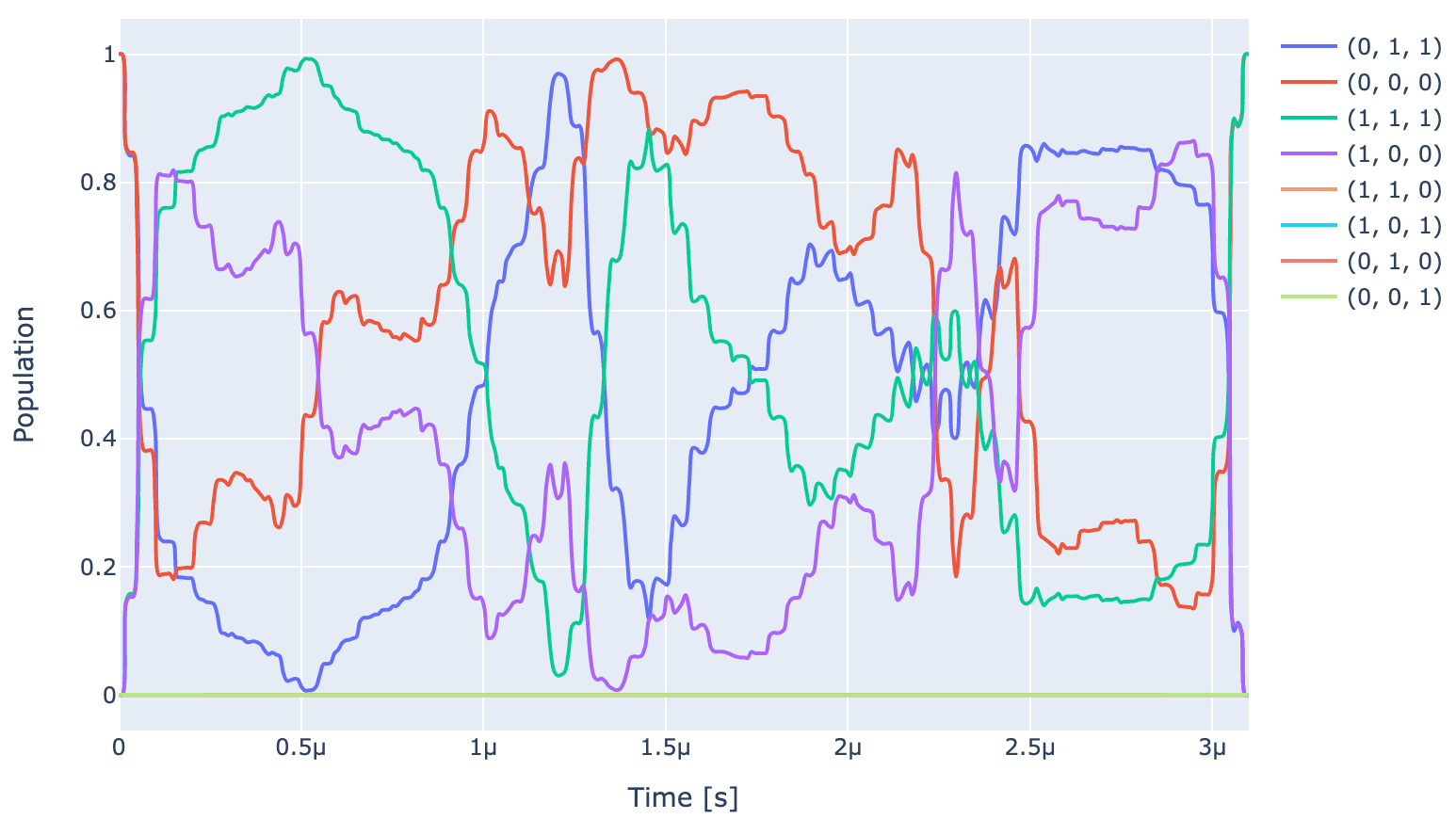
exp.draw_dynamics(Sequence, initial_state)

Expectedly, the population of states $|011\rangle$ and $|111\rangle$ oscillate at the Rabi frequency since carrier frequency is set to be equal to frequency of $|011\rangle \rightarrow |111\rangle$ transition and populations od all the other states oscillate at a detuned frequency. At the end of pulse, under ideal gate, populations of $|011\rangle \leftrightarrow |111\rangle$ and populations of all other states should go back to their initial value. However, as can be seen unoptimized gate (pulse shown below) is not able to achieve that in the provided gate duration.

generator.draw(opt_gate, sim_res, centered=True)

To optimize the pulse, let's set the parameter to be optimized

 drive_opt_map = [
    [(opt_gate.get_key(), "drive_nv", "GRAPE envelope_nv", "inphase")],
    [(opt_gate.get_key(), "drive_nv", "GRAPE envelope_nv", "t_final")],

]

parameter_map.set_opt_map(drive_opt_map)

As done in two qubit gates, we feed the parameter map into OptimalControl object along with setting the cost function, optimization algorithm and Logger. After we run the optimizer, we achieve very high fidelity gate

print(f"Gate Fidelity: {(1 - opt.current_best_goal) * 100} %")
Gate Fidelity: 99.99999985778409 %

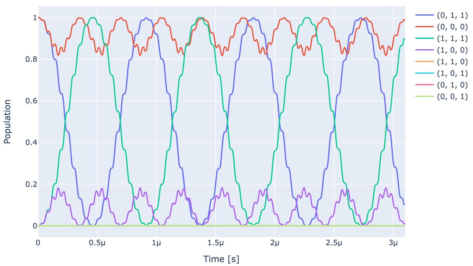
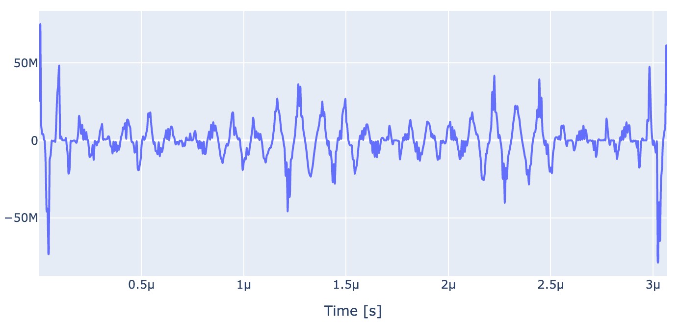
Now let's plot the optimized dynamics and optimized pulse. As we can observe below, the optimized gate is able to produce the expected ideal gate behaviour, i.e., populations of $|011\rangle \leftrightarrow |111\rangle$ and populations of all other states go back to their initial value.

exp.draw_dynamics(Sequence, initial_state)

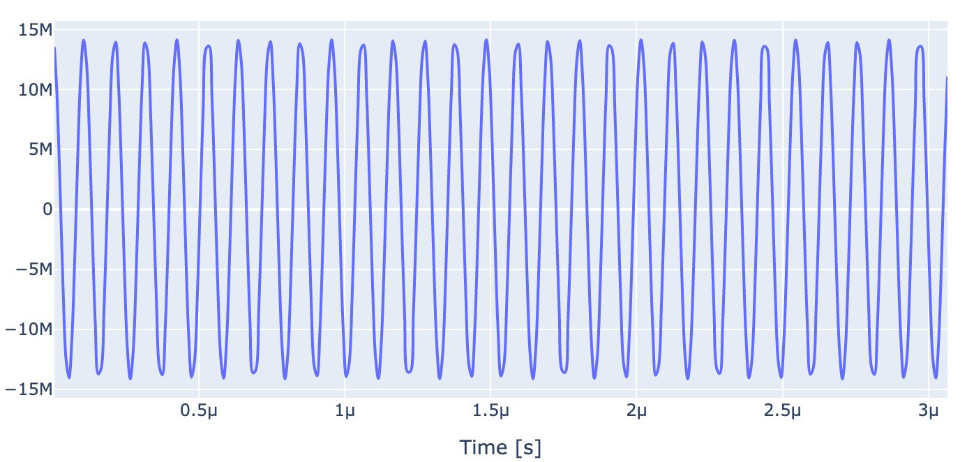
generator.draw(opt_gate, awg_res)

Concluding remarks

To conclude, in this blog post, we demonstrated how to configure a diamond quantum processors using the Qruise toolset and demonstrated high fidelity ( $> 99.99999$ ) unitary gates on it. In our upcoming blog posts, we will demonstrate open loop optimization of a quantum sensing sequence on such a processor.