Getting started with the Qruise toolset

In this blog post, we'll go over one of our introductory notebooks, showing how to set up a simple device with the Qruise toolset and use it for the first step in quantum optimal control. We also have this as the first part of our technical intro tutorials, though we will go into a little more detail here.

Try it yourself

If you're interested in running this tutorial or trying one of our examples of preconfigured devices (superconducting/Rydberg/ion trap/etc) on our demo JupyterHub, fill out our form or email us at demo@qruise.com and we'll get you set up.

Table of Contents

1. Steps in quantum control
2. Device setup: driving a transmon
3. Visualizing the dynamics
4. Open-loop optimal control
5. Concluding remarks

Now, before I get into the details of our device setup, we like to refer to this diagram to explain the steps of quantum optimal control.

1. Steps in quantum control

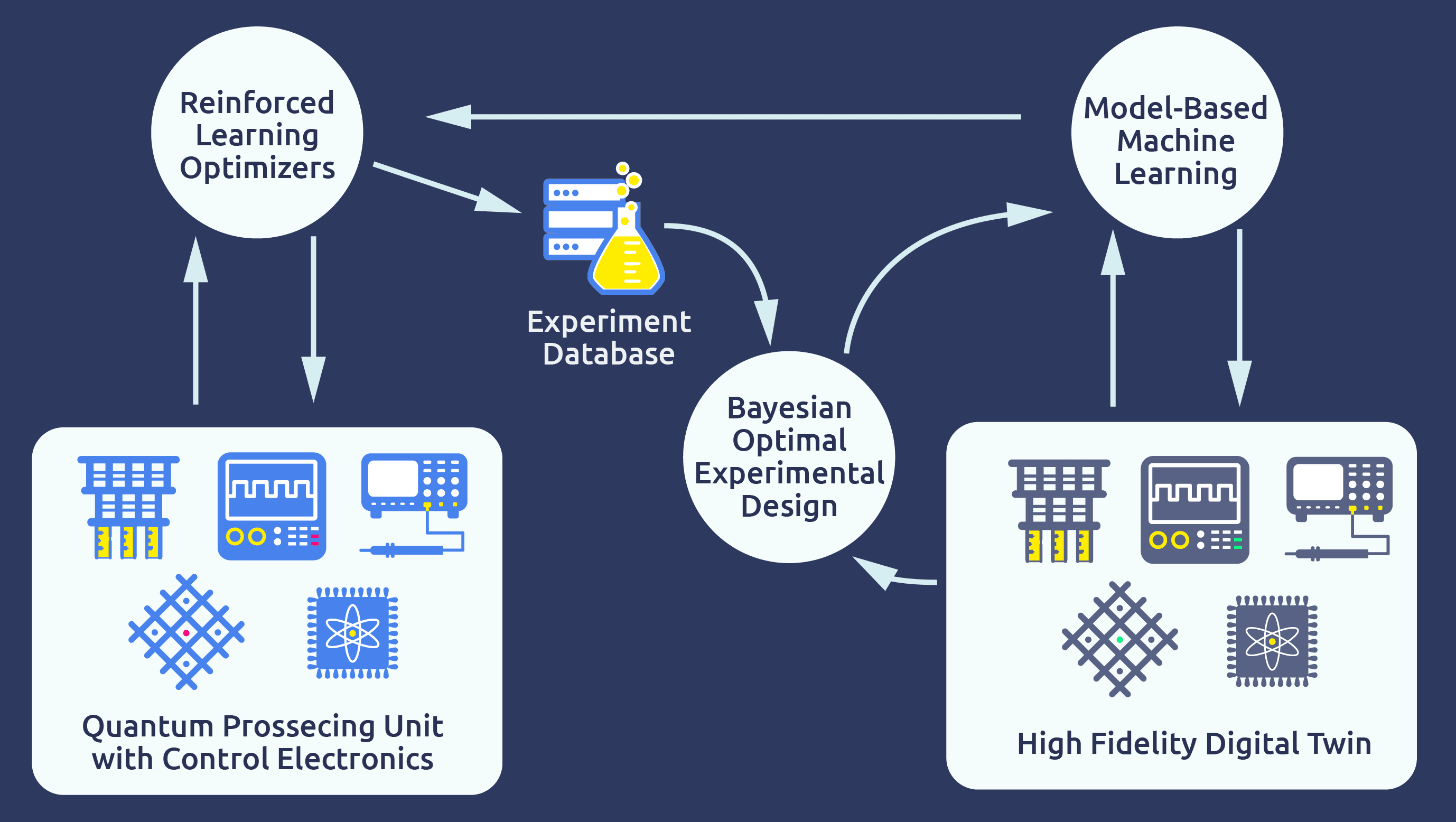
At Qruise, we split up closed-loop quantum optimal control in 3 steps:

• Optimal Control: using a model of the quantum device to run open-loop optimization algorithms to determine control parameters.
• Calibration: adjust control parameters and determine best performance with experiments such as ORBIT on the physical hardware.
• Model Learning: updating the model with the calibration experiments to fix errors and inconsistencies with the model.

In this way, we improve the control and calibration steps in the next iteration, while also nicely separating model based and model-free approaches. In this blog post, I will go through the first step, and in a follow-up post we will go over the other two steps, including how to use Qiskit with the Qruise toolset to interface with physical devices.

So let's set up our single transmon qubit device!

2. Device setup: driving a transmon

As an overview, the device setup process will go in the following steps:

• Model setup: create a model of the components of our device that will also specify the form of the Hamiltonian.
• Signal generation: create a signal generation chain for providing the control pulses accounting for limitations of electronics.
• Instruction set: specify a set of gate instructions for this platform or if needed custom instructions.
• Put it together: and then finally combine these into a simulation environment.

Model setup

As a first step, let's specify some of our key constants and explain them:

import numpy as np # for np.pi and general usage

#transmon constants
freq = 5e9
hilbert_dim = 3
anhar = -210e6
qubit_temp = 0

#Signal generation constants
awg_res = 2e9
sideband = 50e6
lo_freq = freq + sideband

#Gate instruction and basis
t_final = 8e-9  # time for single qubit gates
dressed = True # controls using a dressed basis

So the first part, we will be modeling three-levels of the hilbert space for a transmon qubit (so accounting for one leakage state) with a qubit frequency of 5 GHz, an anharmonicity of -210 MHz, and an idealized temperature of 0K. These values can of course be varied.

For signal generation, we will employ an arbitrary waveform generator with 2 Gigasamples/s (or one pixel per 0.5 ns) for the envelope signal and use a local oscillator with a sideband frequency, so shifted 50 MHz from the qubit resonance.

Finally, we will set our 1-qubit gate times to 8ns and decide to use a dressed basis where we have decided that our computational basis states will be the eigenstates of the time-independent Hamiltonian of our system otherwise known as the drift Hamiltonian and is determined by the Qubit component below.

To input these into a Qruise Model, we define a series of components:

from qruise.toolset.libraries import components, hamiltonians
from qruise.toolset.objects import Quantity as Qty

q1 = components.Qubit(
    name="Q1",
    desc="Qubit 1",
    freq=Qty(freq, 0.999 * freq, 1.001 * freq, unit="Hz 2pi"),
    anhar=Qty(anhar, -380e6, -120e6, unit="Hz 2pi"),
    hilbert_dim=hilbert_dim,
    temp=Qty(qubit_temp, 0.0, 0.12, unit="K"),
)

d1 = components.Drive(
    name="d1",
    desc="Drive on Qubit 1",
    connected=[q1.name],
    hamiltonian_func=hamiltonians.x_drive,
)

---

NOTE

Our Qty or Quantity(value,min_val,max_val,unit) object, is used to represent all parameters of our model, where we (optionally) provide a min and max value. Later, in the optimal control step, we specify which parameters we want to vary within their provided ranges.

---

Qubit Hamiltonian

We model the non-controllable parts of the Hamiltonian in the Qubit component and the controllable part in the Drive component. In general, we support a wide variety of Hamiltonians via a library of specific components such as: Coupling, Transmons, RydbergAtoms, Spins and so forth.

So taking our quantized 2-level Hamiltonian of a transmon qubit our qubit Hamiltonian associated with q1 takes the following form:

$\hat{H}_{\rm tr} = \omega_0 \hat{c}^\dagger \hat{c} + \frac{\delta}{2}\left((\hat{c}^\dagger \hat{c})^2 + \hat{c}^\dagger \hat{c}\right) = \omega_q \hat{c}^\dagger \hat{c} + \frac{\delta}{2}(\hat{c}^\dagger \hat{c})(\hat{c}^\dagger \hat{c} - 1)$

$\hat{c}$ and $\hat{c}^\dagger$ are the transmon annihilation and creation operators $\omega_0 = \sqrt{8 E_c E_J}$ is the ground state frequency $\delta = -E_c$ is the qubit anharmonicity so that $\omega_q = \omega_0 + \delta$ is the so called qubit frequency [ 2 ].

Here $E_c$ is the charging energy and $E_J$ is the Josephson energy, which represent the contributions of the capacitance and non-linear inductance to the quantized Hamiltonian for the superconducting LC circuit [ 2 ] or [ 3 ].

Drive Hamiltonian

Then our drive component d1 has the following simple Hamiltonian after applying the rotating wave approximation (as our detuning between the drive frequency and qubit frequency is small) and then importantly returning to the lab frame:

$\hat{H}_{\rm dr} = -\hbar\Omega \sigma^x$

where $\Omega$ is our drive envelope, which is modeled via the choice of hamiltonians.x_drive for the Drive component.

Now that we have all the parts of our Hamiltonian we combine these to set up our model:

from qruise.toolset.model import Model

model = Model([q1], [d1], dressed=dressed)

---

NOTE

In this example, we will be modeling the Schrödinger equation, but the Qruise toolset also supports modeling the Lindblad master equation, which can be set by adding lindblad=True to the Model args as well as setting t1 and t2star values for the Qubit component.

---

Signal generation

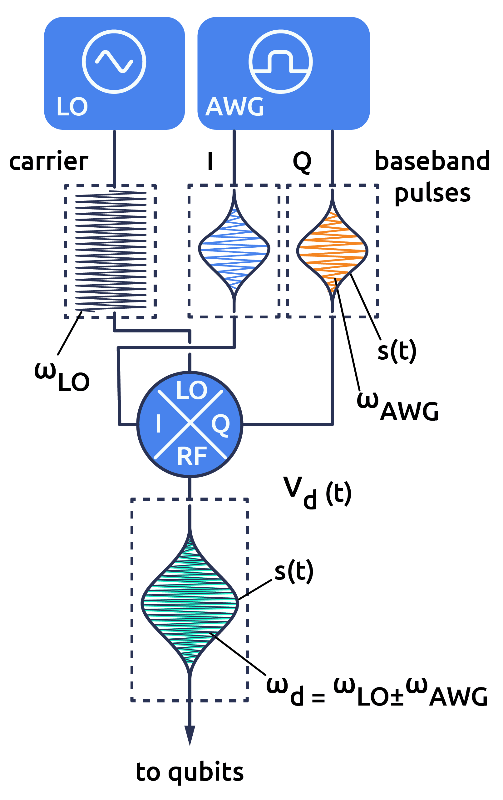
Generally our drive is limited by the performance characteristics of our signal generation chain. We will use the setup shown in the diagram to the right:

• where a local oscillator (LO) determines our drive frequency by creating the carrier signal, while we modulate the amplitude of the drive via an envelope signal.
• the envelope is produced by the combination of an arbitrary waveform generator (AWG) that is limited in its sample frequency (which we specified at the start) and a digital-to-analog converter (DAC).
• the envelope and the carrier are combined together via a mixer to create the oscillating drive signal and finally with the V_to_Hz device below converts the voltage of the signal to the frequency scale of the qubit.

In the Qruise toolset, one can specify other signal generation setups and also add noise characteristics, via our library of generator devices. For this intro we will stick with our SimpleGenerator setup, which assumes no noise or harmonics are introduced in the signal generation chain:

from qruise.toolset.generator.generator import SimpleGenerator

generator = SimpleGenerator(
    V_to_Hz=Qty(value=1e9, min_val=0.9e9, max_val=1.1e9, unit="Hz/V"),
    awg_res=awg_res,
)

---

NOTE

As an aside, the characteristics of the signal generation process are particularly important when using high parameterized pulse shapes (such as piecewise constant). This is because the sample frequency of the AWG is of a similar magnitude to the transmon frequency and thereby our drive frequency, so the envelope shapes that an AWG can generate within one wavelength are limited.

---

Instruction set

Now that we have specified both the form of our Hamiltonian and the signal generation chain, we need to specify the control parameterization of the drive envelope and associate our control parameters to some ideal instruction (gate) that we are targeting. In this tutorial, I will be configuring $\frac{\pi}{2}$-pulses otherwise known as R90 gates and will use a Gaussian envelope, but the Qruise toolset has a library of many parameterization schemes including piecewise constant (PWC) parameterizations as well, as is used for the GRAPE algorithm.

First, we define our Instruction and provide the ideal gate unitary, which takes the form of a 2x2 numpy array, as it is a single-qubit gate and is only defined for the 2 computational basis states. Here I define the $R_x(\frac{\pi}{2})$ gate.

from qruise.toolset.signal.gates import Instruction
from qruise.toolset.libraries import constants

rx90p = Instruction(
    name="rx90p", t_end=t_final, channels=[d1.name], targets=[0], ideal=constants.x90p
)

Specify control parameterization

Now that we have an instruction, we need to specify our control parameters for both the carrier and the envelope.

from qruise.toolset.signal.pulse import Carrier, Envelope
from qruise.toolset.libraries import envelopes

carrier_parameters = {
    "freq": Qty(lo_freq, 4.5e9, 6e9, unit="Hz 2pi"), # carrier frequency determined by LO
    "framechange": Qty(0.0, -np.pi, 3 * np.pi, unit="rad"), # carrier phase at start
}

rx90p.add_component(Carrier(
    name="carrier",
    desc="Frequency of the local oscillator",
    params=carrier_parameters,
))

gauss_params_single = {
    "amp": Qty(0.45, 0.3, 0.5, unit="V"), # envelope amplitude in V as non-normalised
    "t_final": Qty(t_final, 0.5 * t_final, 1.5 * t_final, unit="s"), # time of the pulse, matches gate time
    "sigma": Qty(0.25 * t_final, 0.125 * t_final, 0.5 * t_final, unit="s"), # std deviation of the gaussian
    "xy_angle": Qty(0.0, -0.5 * np.pi, 2.5 * np.pi, unit="rad"), # controls inphase and quadrature of envelope for X or Y gate application
    "freq_offset": Qty(-sideband, unit="Hz 2pi"), # accounts for drive frequency being offset from qubit frequency
    "delta": Qty(-1, -1.01, -0.49, unit=""), # controls application of DRAG procedure
}

rx90p.add_component(Envelope(
    name="gauss",
    desc="Gaussian comp for single-qubit gates",
    params=gauss_params_single,
    shape=envelopes.gaussian_nonorm,
))

A brief note on the delta parameter. It enables usage of the DRAG procedure to reduce dephasing and leakage errors by applying a derivative of the envelope to the out-of-phase component. It is dimensionless and is the negative of what is sometimes referred to as $\lambda$ and is set between -1 and -0.5.

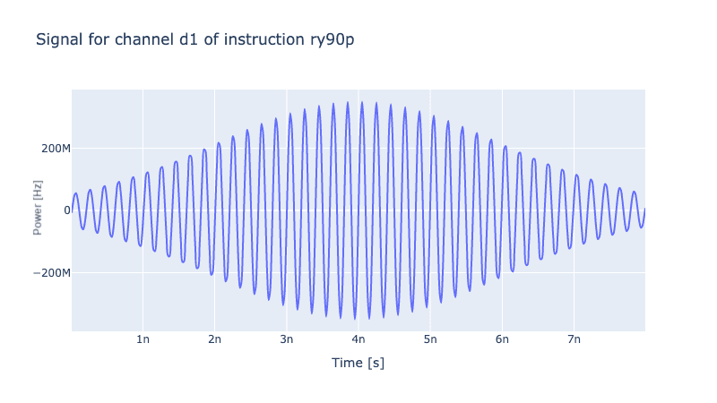
Now that we have associated control parameters to a specific instruction, one can plot the signal for the current parameter values to get some intuition (the y-axis is in the frequency scale of the qubit, divide by $10^9$ to get volts):

generator.draw(rx90p, 10 * lo_freq)  # x10 to prevent aliasing in the plot

Additional instructions

For convenience one can copy one instruction and only specify the modified parameter values. For example, to get the other R90 gates, so $R_y(\frac{\pi}{2})$, $R_x(\frac{-\pi}{2})$, and $R_y(\frac{-\pi}{2})$, we change the xy_angle by factors of $\frac{\pi}{2}$, to change the relative phase of the drive local oscillator and the transmon. Another way to describe this is that it is shifting the trajectory on the Bloch sphere for the gate dynamics by $\frac{\pi}{2}$ and so shifting the axis of rotation along the equator between the X and Y axes.

ry90m = rx90p.copy(name="ry90m",
                   ideal=constants.y90m,
                   params={("d1","gauss","xy_angle"): Qty(0.5 * np.pi,
                                                          -0.5 * np.pi, 2.5 * np.pi, unit="rad")}
                   )
rx90m = rx90p.copy(name="rx90m",
                   ideal=constants.x90m,
                   params={("d1","gauss","xy_angle"): Qty(1.0 * np.pi,
                                                          -0.5 * np.pi, 2.5 * np.pi, unit="rad")}
                   )
ry90p = rx90p.copy(name="ry90p",
                   ideal=constants.y90p,
                   params={("d1","gauss","xy_angle"): Qty(1.5 * np.pi,
                                                          -0.5 * np.pi, 2.5 * np.pi, unit="rad")}
                   )

Putting it all together

Now let's make a list of the configured instructions and then use that momentarily to create the simulation environment.

instructions = [rx90p,
                ry90m,
                rx90m,
                ry90p
                QId,  # optional, comment out if not set
                ]

We now combine the model, generator, and instructions into what we call the ParameterMap and it is what one typically as a user interfaces with as it combines all the variables and parameters we just configured. Using that, we also set up the simulation Environment.

from qruise.toolset.parametermap import ParameterMap
from qruise.toolset.experiment import Experiment

parameter_map = ParameterMap(
    model=model, generator=generator, instructions=instructions
)
sim_res = 1e11 # some value for the simulation frequency that is higher than the dynamics frequency we expect to see, usually between 1e10 and 1e11 for superconducting qubits.
simulation = Experiment(pmap=parameter_map, sim_res=sim_res)

Here the simulation frequency determines the time step resolution used to simulate the time evolution dynamics.

Yay! We now have a fully configured simulation, so let's plot some dynamics of the system.

3. Visualizing the dynamics

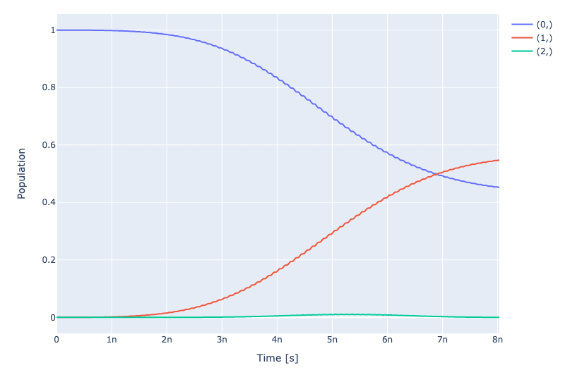
To investigate the dynamics, we define the initial state of the system to be in the ground state: $|0\rangle$ and then specify the instructions we want to simulate. I'll use rx90p[0] which is how we specify the rx90p gate with the 0th qubit as target.

initial_state = np.array([1,0,0])  # can also use model.get_ground_state()
barely_a_seq = ["rx90p[0]"]  # can also use rx90p.get_key()

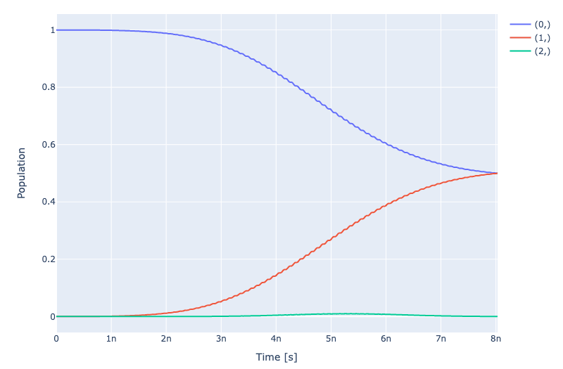
simulation.draw_dynamics(sequence=barely_a_seq, state=initial_state)

Here the y-axis is the population of each of the states over the course of the simulation. As you can see while the leakage to the $|2\rangle$ state rises slightly, the final state is not in an equal superposition of $|0\rangle$ and $|1\rangle$. This is due to the un-optimized control parameters, as the pulse has overshot the $\frac{\pi}{2}$ rotation. We will fix this in the optimal control step.

4. Open-loop optimal control

To specify an optimal control task, we need to:

• Specify the instruction set: specify which instructions we want to optimize, in this case it will be the 4 R90 gates.
• Specify control parameters: specify the subset of control parameters that we want to vary in the optimization
• Run optimal control: specify a suitable goal function we want to minimize, in this case it will be the unitary infidelity, so one minus the unitary overlap: $1 - Tr[U_{sim},U_{ideal}^\dagger]$. Then use that to run the optimal control task.

Specify the instruction set

To specify the instructions one runs:

simulation.set_opt_gates(["rx90p[0]","ry90m[0]","rx90m[0]","ry90p[0]"])

Specify control parameters

To specify the subset of control parameters one runs:

opt_map = [
    # each set of 4 shares the same value between the 4 r90 gates
    parameter_map.find_keys("gauss","amp"),
    parameter_map.find_keys("gauss","delta"),
    parameter_map.find_keys("gauss","sigma"),
]
parameter_map.set_opt_map(opt_map)

Here, we are specify the parameters using a tuple: (instr_name,channel_name,component_name,param_name), such as ("rx90p[0]", "d1", "gauss", "amp"). The find_keys command finds all keys that match the subset of parts and groups them together, so we will use the same amplitude parameter (amp) for all 4 gates.

So expanded the opt_map looks like:

opt_map
[
    [
        'rx90p[0]-d1-gauss-amp',
        'ry90p[0]-d1-gauss-amp',
        'rx90m[0]-d1-gauss-amp',
        'ry90m[0]-d1-gauss-amp'
    ],
    [
        'rx90p[0]-d1-gauss-delta',
        'ry90p[0]-d1-gauss-delta',
        'rx90m[0]-d1-gauss-delta',
        'ry90m[0]-d1-gauss-delta'
    ],
    ...
]

A cleaner way to view it is via the parameter_map.print_parameters() command, which also groups the parameters sharing the same value together.

rx90p[0]-d1-gauss-amp                 : 350.000 mV
ry90p[0]-d1-gauss-amp
rx90m[0]-d1-gauss-amp
ry90m[0]-d1-gauss-amp

rx90p[0]-d1-gauss-delta               : -1.000 V
ry90p[0]-d1-gauss-delta
rx90m[0]-d1-gauss-delta
ry90m[0]-d1-gauss-delta

rx90p[0]-d1-gauss-freq_offset         : -50.000 MHz 2pi
ry90p[0]-d1-gauss-freq_offset
rx90m[0]-d1-gauss-freq_offset
ry90m[0]-d1-gauss-freq_offset

rx90p[0]-d1-carrier-framechange       : 0.000 rad
ry90p[0]-d1-carrier-framechange
rx90m[0]-d1-carrier-framechange
ry90m[0]-d1-carrier-framechange

Run optimal control

Now that the set of control parameters and set of instructions are provided via the parameter_map, we can run the actual optimal control algorithm. One key advantage of the Qruise toolset is that we support both gradient based and gradient-free optimization algorithms via our integration with the Tensorflow framework, so in this case, we will use L-BFGS algorithm for a gradient based optimization. (We are also working on ML optimization algorithms.)

The snippet below both configures and runs the optimal control optimization. Here the import of lbfgs is a small wrapper around the SciPy L-BFGS function and the fid_func is the unitary infidelity as mentioned before.

from qruise.toolset.optimizers.optimalcontrol import OptimalControl
from qruise.toolset.optimizers.loggers import PlotLineChart
from qruise.toolset.libraries.fidelities import unitary_infid_set
from qruise.toolset.libraries.algorithms import lbfgs

opt = OptimalControl(
    fid_func=unitary_infid_set,
    fid_subspace=[q1.name],  # selects the target qubit, important in larger models
    pmap=parameter_map,
    algorithm=lbfgs,
    options={"maxfun": 100},
    logger=[PlotLineChart()],  # show us a nice progress plot :)
)
opt.set_exp(simulation)

opt.run()  # starts the optimal control optimization

This will start printing out logging messages and a plot like this. Since we are minimizing infidelity we want the goal function to be near 0, which it is:

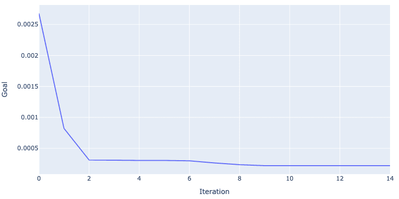
print(opt.current_best_goal)
0.0002205864641723343

This gives a fidelity of 99.978%. Looking at the dynamics plot below we see a near perfect equal superposition of $|0\rangle$ and $|1\rangle$, with the remaining infidelity due to leakage to the $|2\rangle$.

simulation.compute_propagators()  # updates the simulation with the new parameter values
simulation.draw_dynamics(sequence=barely_a_seq, state=initial_state)

We have optimized the amplitude, sigma and DRAG delta parameter to minimize the leakage and at the expense of increasing t_final slightly one can suppress the leakage even further.

parameter_map.print_parameters()

rx90p[0]-d1-gauss-amp                 : 347.213 mV
ry90p[0]-d1-gauss-amp
rx90m[0]-d1-gauss-amp
ry90m[0]-d1-gauss-amp

rx90p[0]-d1-gauss-delta               : -0.898
ry90p[0]-d1-gauss-delta
rx90m[0]-d1-gauss-delta
ry90m[0]-d1-gauss-delta

rx90p[0]-d1-gauss-sigma               : 1.877 ns
ry90p[0]-d1-gauss-sigma
rx90m[0]-d1-gauss-sigma
ry90m[0]-d1-gauss-sigma

5. Concluding remarks

Excellent, we have a fully configured device and were able to run optimal control to update the control parameters.

In our next tutorial we will go over the calibration and model learning steps, where we update the control parameters and the model to account for unknown values and noise characteristics of the model.

Also, be on the lookout for additional tutorials where we will go through working with different qubit architectures and working with larger systems. I will also give a tutorial going through some of the different propagation methods we support for our simulations.

Thanks for following along :)

Citations

1 J. Kelly et al., “Optimal Quantum Control Using Randomized Benchmarking,” Physical Review Letters, vol. 112, no. 24, Jun. 2014, doi: 10.1103/physrevlett.112.240504.

2 Qiskit, “Introduction to Transmon Physics,” Nov. 29, 2022. https://qiskit.org/textbook/ch-quantum-hardware/transmon-physics.html

3 A. Blais, A. L. Grimsmo, S. M. Girvin, and A. Wallraff, “Circuit Quantum Electrodynamics”, Reviews of Modern Physics, 93, 025005, May 2021, doi: 10.1103/RevModPhys.93.025005

4 F. Motzoi, J. M. Gambetta, P. Rebentrost, and F. K. Wilhelm, “Simple Pulses for Elimination of Leakage in Weakly Nonlinear Qubits,” Physical Review Letters, vol. 103, no. 11, Sep. 2009, doi: 10.1103/physrevlett.103.110501.