Taming the Unimons

Products & Services

Resources

News & Events

Company

Book a demo

All blog posts

Taming the Unimons

Abstract

Unimons belong to the class of superconducting qubits. They exhibit an enhanced anharmonicity compared to transmons. At the same time, they are fully isolated against dc charge noise and show lower sensitivity to flux noise. In this post, we demonstrate how one can model the Unimons within the Qruise ecosystem and simulate their dynamics upon the action of single-qubit gates. Moreover, we give an overview on how to couple two unimons and entangle them using the Qruise toolset and perform the CNOT gate on such a 2-qubit system. The results reported here confirm that the fidelity of single-qubit gates, e.g. $RX(\pi/2)$ gate with a pulse duration of 7 ns pulse is 99.99%. The same fidelity is yielded for the CNOT gate with a pulse duration of 50 ns. We introduce as well a two-stage optimal control protocol to enhance the fidelity of more sophisticated gate instructions.

Table of Content

Abstract
1. Concise Introduction to Unimons
- 1.1 Unimon Hamiltonian
2. Unimons in Qruise Toolset
References

1. Concise Introduction to Unimons

Unimons are superconducting qubits designed in a collaboration between Aalto University and VTT Technical Research Centre [1]. It is a superconducting circuit in which a single Josephson junction is integrated into the centre conductor of a superconducting coplanar-waveguide (CWP). It is characterised by seven parameters, the length $(l)$ , capacitance per unit length density $(C_l)$ , inductance per unit length density $(L_l)$ of the circuit and the characteristics of the Josephson junction, namely Josephson capacitance $(C_J)$ , Josephson inductance $(L_J)$ and the location $(x_J)$ of the Josephson junction. Moreover, the background flux bias $\Phi_{\rm diff}$ affects the dc flux of the Josephson junction, subsequently affecting the Hamiltonian of the system.

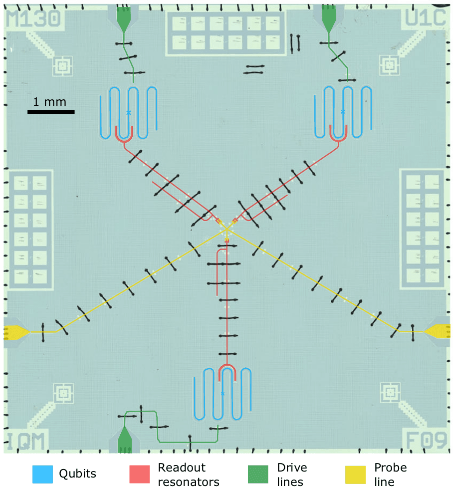
Fig. 1 A silicon chip with three unimons, their drive lines, readout resonators and probe lines. The image is adapted from Ref. [1]

In the figure above, the unimons are shown with blue colour. The cross at the centre of each unimon depicts the location of the Josephson junction. One can model the unimon using the distributed-element circuit model by discretising the CWP into $N$ inductors of magnitude $L_l\Delta x$ and capacitors of magnitude $C_l\Delta x$ , where $\Delta x = l/N$ [1, 2].

1.1 Unimon Hamiltonian

To derive the expression describing the Hamiltonian of a unimon with the parameters defined above, one needs to solve the Lagrangian for the canonical coordinates $\Psi_i$ 's of the discretised circuit shown in the figure below.

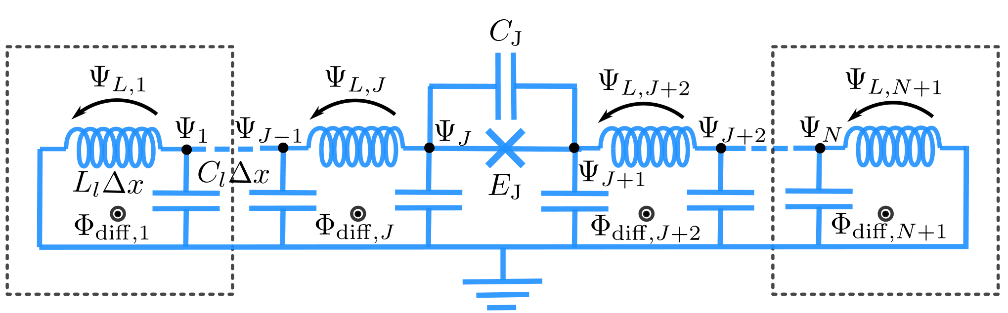
Fig. 2 Distributed-element circuit model after discretisation (See Ref.[1, 2]). Each element $i$ has the inductance of $L_l\Delta x$ and capacitance of $C_l\Delta x$ . It will be shown that the flux difference bias $\Phi_{\rm diff}$ plays a crucial role in the enhancement of the anharmonicity of the unimon. The image is taken from the supplementary material of Ref.[1].

The kinetic and potential energies associated with the canonical coordinates $\Psi_i$ 's yield the followings

$\begin{aligned} & T = \sum_{i=1}^N \frac{1}{2}C_l\Delta x\dot{\Psi}_i^2 + \frac{1}{2}C_J(\dot{\Psi}_{J+1} - \dot{\Psi}_J)^2, \\ & U = \frac{1}{2L_l\Delta x} \sum_{i=1\neq J+1}^{N+1} (\Psi_{i-1} - \Psi_i + \Phi_{\mathrm{diff},i})^2 - E_J\cos\left[\frac{2\pi}{\Phi_0}(\Psi_{J+1}-\Psi_J)\right] \end{aligned}$

where $\Psi_J$ and $\Psi_{J+1}$ are the Lagrangian canonical coordinates at the boundaries of the Josephson junction, and $\Phi_0$ is the flux quanta. The background flux bias $\Phi_{\mathrm{diff},i}$ for each element can be set to be $\Phi_{\rm diff}$ under the assumption that the background flux bias is homogeneous.

Solving the Lagrange equation and taking the continuum limit, i.e. $\Delta x \rightarrow 0$ , one arrives at the following wave solution for $\psi(x,t)$ (solution of $\Psi_i$ in the continuum limit).

$\ddot{\psi}(x, t) = v^2\partial_{xx}\psi(x,t),$

where $v = 1/\sqrt{L_l C_l}$ is the wave velocity. The equation above admits the following general solution

$\psi(x,t) = \phi_0 u_0(x) + \sum_{m\geq 1} u_m(x)\psi_m(t),$

with $\phi_0$ the flux difference across the Josephson junction contributing to the dc component with its envelope $u_0(x)$ , and the summation part that contributes to the ac oscillations of the flux which consisting of $\psi_m(t) = \exp(-i\omega_m t)$ oscillations where $\omega_m$ is the classical frequency of the mode $m$ and its envelope $u_m(x)$ .

The wave solution must satisfy the current continuity condition across the Josephson junction. This is implied by the following expression deduced after solving the Lagrange equation for $\Psi_i$ 's.

$\begin{aligned} -C_J\Delta\ddot{\psi} - I_c\sin\left(\frac{2\pi}{\Phi_0}\Delta\psi\right) = -\frac{1}{L_l}\partial_x\psi\Big|_{x=x_J^-} + \frac{\Phi_{\rm diff}}{2lL_l}, \end{aligned}$

where $I_c$ is the super-current of the Josephson junction given by $\Phi_0/(2\pi L_J)$ which subsequently yields the following three independent equations after inserting $\psi(x,t)$ into the continuity equation above.

$\begin{aligned} & I_c\sin\left(\frac{2\pi}{\Phi_0}\phi_0\right) + \frac{\phi_0}{2lL_l} = \frac{\Phi_{\rm diff}}{2lL_l} &&&& (1)\\ & \omega_m^2C_J\Delta u_m - \frac{\cos(2\pi\phi_0/\Phi_0)}{L_J}\Delta u_m = -\frac{1}{L_l}\partial_x u_m\Big|_{x=x_J^-} &&&& (2)\\ &-\frac{1}{L_l}\partial_x u_m\Big|_{x=x_J^-} = -\frac{1}{L_l}\partial_x u_m\Big|_{x=x_J^+} &&&& (3) \end{aligned}$

It is worth mentioning that this set of equations is only valid under the assumption of small ac oscillations. This leads to the linearisation of the current continuity equation around the dc component of the wave solution, which consequently leads to the decoupling of different modes of the wave solution.

1.1.1 Solution to the Josephson Flux

In the set of equations satisfying the current continuity condition, the transcendental Eq. (1) yields the solution for $\phi_0$ . We can plot the solution by calling the unimon.vis.plot_josephson_flux. It is interesting to observe that at the sweet spot $\Phi_{\rm diff} = \Phi_0/2$ the solution to this transcendental equation yields $\varphi_0 = 2\pi\phi_0/\Phi_0 = \pi$ .

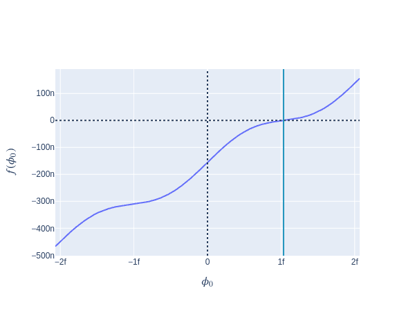
Fig. 3 The solution to $\phi_0$ given by the transcendental Eq. (1). The vertical line shows the intersection of the curve governing the behaviour of $\phi_0$ and the constant vertical line given by $\Phi_{\rm diff}/(2lL*l)$ .

In the plot above we see how the transcendental Eq. (1) behaves around the origin. It is straightforward to check that the solution (the intersection of the curve and the vertical line) is given by $\Phi_0/2$ .

For the envelope of the dc component to comply with this equation, it must behave as a piece-wise linear function given by

$\begin{aligned} u_0(x) = \begin{cases} (x+l)/2l & \text{if} & -l\leq x < x_J\\ (x-l)/2l & \text{if} & x_J < x \leq l \end{cases}. \end{aligned}$

1.1.2 Solution to the Envelope of the AC Oscillations

On the other hand, the envelopes of the ac component must, in their most general form, admit a piece-wise sinusoidal function i.e.

$u_m(x) = \begin{cases} A_m\sin[k_m(x+l)]& \text{if} & -l\leq x < x_J\\ A_mB_m\sin[k_m(x-l)]& \text{if} & x_J < x \leq l, \end{cases}.$

where $k_m = \omega_m / v$ is the wave number of mode $m$ . By substituting the expression above in Eq.(3), one solves for the dimensionless factor $B_m$ .

$\begin{aligned} B_m = \frac{\cos[k_m(x_J +l)]}{\cos[k_m(x_J - l)]}.\end{aligned}$

Yet, the solution for the dimensionless factor $A_m$ is a bit more involved. To arrive at the solution, one has to use the fact that $u_m(x)$ 's are orthogonal i.e.

$\langle u_m(x) u_n(x) \rangle = \int_{-l}^{l} C_l u_m(x) u_n(x) dx + C_J\Delta u_m \Delta u_n = C_{\Sigma}\delta_{mn},$

where $C_{\Sigma} = 2lC_l + C_J$ and $\Delta u_m$ is the difference of the envelope amplitude at $x_J^+$ and $x_J^-$ . Asserting the condition that $u_m$ 's to be orthonormal, one arrives at the following expression for $A_m$

$\begin{aligned} A_m = \Bigg\{&\frac{C_l}{2C_{\Sigma}}\left[(x_J + l) - \frac{\sin[(2k_m(x_J + l))]}{2k_m}\right] + \frac{C_J}{2C_{\Sigma}}\bigg[1 - \cos[2k_m(x_J + l)]\bigg] + \\ &\frac{C_lB_m^2}{2C_{\Sigma}}\left[(l-x_j) + \frac{\sin[2k_m(x_J - l)]}{2k_m}\right] + \frac{C_JB_m^2}{2C_{\Sigma}}\bigg[1-\cos[2k_m(x_J-l)]\bigg] - \\& \frac{4C_JB_m}{C_{\Sigma}}\bigg[\cos(2k_mx_J) - \cos(2k_ml)\bigg]\Bigg\}^{-1/2}\end{aligned}$

1.1.3 Solution to the Wavenumber

For $A_m$ and $B_m$ to be known exactly, one needs to know $k_m$ which itself requires one to know $\phi_0$ . The value of $\phi_0$ is already known via Eq.(1). Substituting that along the solution of $B_m$ into Eq.(2) one arrives at the following transcendental equation for $k_m$

$\begin{aligned} g(k_m) = k_m l \cos[k_m(x_J - l)]\cos[k_m(x_J + l)] - \left[\frac{(k_m l)^2C_J}{C_l l} - \frac{L_l l}{L_J}\cos\left(\frac{2 \pi \phi_0}{\Phi_0}\right)\right]\sin(2k_m l). \end{aligned}$

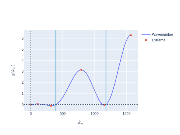
Fig. 4 Curve depicting the behaviour of $g(k_m$ . Solutions are classified to the modes of even and odd numbers. The location of the vertical lines hints at wave solutions with the mode number even

In the figure above, one classifies the solutions of $k_m$ into two distinct groups, ones that refer to the wave number that their mode number is odd and the others that their mode is even. The vertical lines show the solution of $k_m$ with $m\in\mathbb{Z}/2\mathbb{Z}$ .

By having the values of $k_m$ , $A_m$ and $B_m$ known, one arrives at the exact analytical solution of $u_m$ . Knowing $u_m$ is crucial to know the characteristic parameters of the Hamiltonian of a single unimon, which will be elaborated on shortly.

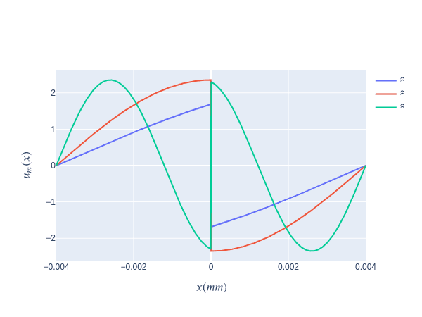
Fig. 5 Envelope of the ac component of the wave solution for the first three modes at the sweet spot. At the Josephson junction $x=0$ , the envelope changes signs.

The figure above depicts the solution of $u_m$ for three different modes, namely 1, 2, and 3. It is evident that at the boundary condition where the Josephson junction is located, the envelope changes sign abruptly. Yet, the derivative of the curve remains continuous, satisfying the boundary condition of the wave equation.

1.1.4 The Hamiltonian of a Single Unimon

We saw that the wave solution involves an infinite sum over the normal modes of the ac oscillations. Nevertheless, one can approximate the solution up to a single mode and discard the rest. It is essential to know that for more precise numerical analysis, summation over modes up to a certain threshold may be required. Yet, for the time being, consider the single mode approximation, i.e. $\psi(x,t) = \phi_0u_0(x) + u_m(x)\psi_m(t)$

The Lagrangian is then read as

$\begin{aligned} \mathcal{L} = \frac{C_m^\prime}{2}\dot{\phi}_m^2 - \frac{1}{2\tilde{L}^\prime_m}\phi_m^2 - \frac{1}{2lL_l}(\Phi_{\rm diff}-\phi_0)\phi_m + E_J\cos\left[\frac{2\pi}{\Phi_0}(\phi_m - \phi_0)\right], \end{aligned}$

with the flux variable $\phi_m = \psi_m\Delta u_m$ , $C_m^\prime = C_\Sigma/(\Delta u_m)^2$ , and $\tilde{L}_m^\prime = \tilde{L}_m(\Delta u_m)^2$ . The total capacitance is $C_\Sigma = C_J + 2lC_l$ , and the effective inductance $\tilde{L}_m(\phi_0)$ is given by

$\begin{aligned} \frac{1}{\tilde{L}_m(\phi_0)} = \frac{1}{L_m} - \frac{\cos(2\pi\phi_0/\Phi_0)}{L_J}(\Delta u_m)^2, \end{aligned}$

where $L_m = (C_\Sigma\omega_m^2)^{-1}$ . By taking the Legendre transformation of the Lagrangian above, the following Hamiltonian is deduced.

$\begin{aligned} H_m = \frac{q_m^2}{2C_m^\prime} + \frac{\phi_m^2}{2\tilde{L}_m^\prime} + \frac{1}{2lL_l}(\Phi_{\rm diff}-\phi_0)\phi_m - E_J\cos\left[\frac{2\phi}{\Phi_0}(\phi_m - \phi_0)\right] \end{aligned}$

where $q_m = \partial\mathcal{L}/\partial\dot{\phi}_m$ is the canonical conjugate momentum of the flux variable $\phi_m$ . The Poisson bracket of $q_m$ and $\phi_m$ is unity, i.e. $\{\phi_m, q_m\} = 1$ . Hence we can introduce their quantum counterpart variables that satisfy the commutation relation $[\hat{\phi_m}, \hat{q_m}] = i\hbar$ . Introducing the dimensionless operators $\hat{n}_m$ and $\hat{\varphi}_m$ that satisfy the commutation relation $[\hat{\varphi}_m, \hat{n}_m] = i$ , the Hamiltonian above can be rewritten as

$\begin{aligned} \hat{H_m} = 4E_{C,m}(\varphi_0)\hat{n}_m^2 + \frac{1}{2}E_{L,m}(\varphi_0)\hat{\varphi}_m^2 + E_L(\varphi_{\rm diff}-\varphi_0)\hat{\varphi}_m - E_J\cos(\hat{\varphi}_m - \varphi_0), \end{aligned}$

with $E_{C,m}(\varphi_0) = e^2/2C_m^\prime$ , $E_{L,m} = (\Phi_0/(2\pi))^2/\tilde{L}_m^\prime$ , $E_L = (\Phi_0/(2\pi))^2/(2lL_l)$ , and $\varphi_{\rm diff} = 2\pi\Phi_{\rm diff}/\Phi_0$ .

The classical potential associated with the flux (phase) operator $\hat{\varphi}_m$ is shown below

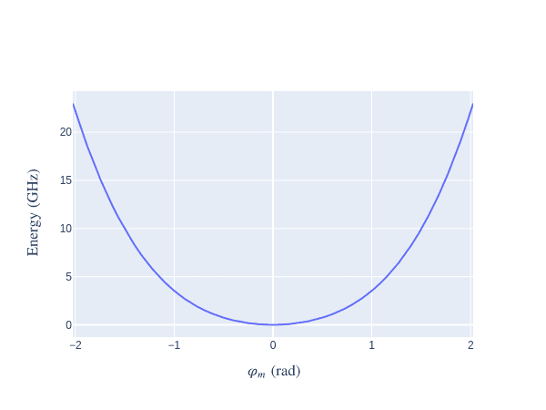
Fig. 6. The potential associated with the flux operator $\hat{\varphi}_m$ around the origin.

As mentioned earlier, at the sweet spot $\varphi_0 = \pi = \varphi_{\rm diff}$ which simplifies the Hamiltonian above to the following simple form

$\begin{aligned} \hat{H}_m = 4E_{C,m}(\varphi_0)\hat{n}_m^2 + \frac{1}{2}E_{L,m}\hat{\varphi}_m^2 + E_J\cos(\hat{\varphi}_m). \end{aligned}$

Assuming that $||\varphi_m||\ll 1$ , one can expand the cosine function up to $\mathcal{O}(\hat{\varphi}_m^6)$ which leads to the following expression for the Hamiltonian,

$\begin{aligned} \hat{H}_m = 4E_{C,m}(\varphi_0)\hat{n}_m^2 + \frac{1}{2}(E_{L,m} - E_J)\hat{\varphi}_m^2 + \frac{E_J}{4!}\hat{\varphi}_m^4 + \mathcal{O}(\hat{\varphi}_m^6) \end{aligned}$

If designed precisely, $E_{L,m}$ and $E_J$ cancel out each other, and the second order term vanishes. Hence, one is left only with the quartic term. This enhances the anharmonicity greatly in the unimons compared to transmons.

Introduce $\alpha = \sqrt{4E_{C,m}}$ and $\beta = \sqrt{(E_{L,m} - E_J)/2}$ , and write the charge and flux operators in terms of the ladder operators $a$ and $a^\dagger$ as

$\begin{aligned} \hat{n}_m = -\frac{i}{2}\left(\frac{2\beta}{\alpha}\right)^{1/2}(a - a^\dagger)\\ \hat{\varphi}_m = \frac{1}{2}\left(\frac{2\alpha}{\beta}\right)^{1/2}(a + a^\dagger) \end{aligned}$

Such a substitution let one write the simplified Hamiltonian above in terms of the ladder operators as

$\begin{aligned} \hat{H}_m = 2\alpha\beta\left(a^\dagger a + \frac{1}{2}\right) - \frac{E_J}{4!4}\left(\frac{\alpha}{\beta}\right)^2(a + a^\dagger)^4 \end{aligned}$

Using the fast rotating approximation the last term can be simplified which ultimately leads to the following expression for the Hamiltonian

$\begin{aligned} \hat{H}_m = \gamma\left(\frac{\zeta}{\gamma}\bm{1} - a^\dagger a\right)a^\dagger a, \end{aligned}$

where $\gamma = E_J/16(\alpha/\beta)^2$ and $\zeta = 2\alpha\beta - \gamma$ . The Hamiltonian above resembles the one of Duffing oscillator.

Now that we have the Hamiltonian, we can proceed with building the Unimon circuit and the electronics components, such as AWG, Mixer, drive line, etc. to introduce gate instructions and manipulate our unimon. Finally, we will show how to perform optimal control on these gate instructions to achieve high gate fidelities. Here we assume that the reader is already familiar with the Qruise toolset and how each component is attached to one another within the Qruise ecosystem. It is highly recommended to read this introductory blog post before proceeding if you feel uncomfortable with the Qruise toolset. Moreover, for an in-depth and extended review of the qubit circuitry refer to Ref.[3].

2. Unimons in Qruise Toolset

2.1 Instantiating a Unimon Qubit

A unimon is defined in the Qruise toolset by calling the Unimon class and passing the parameters mentioned earlier that characterise the unimon qubit. We define some of the parameters of our system and then create a Unimon object as shown below:

hilbert_dim=3
params ={
    "length": Quantity(
        value=4.0e-3, min_val=3.9e-3,
        max_val=4.1e-3, unit="m"),
    # The capacitance density per unit length
    "capacitance_den": Quantity(
        value=83e-12, min_val=80e-12,
        max_val=86e-12, unit="F/m"),
    # The inductance density per unit length
    "inductance_den": Quantity(
        value=0.83e-6, min_val=0.80e-6,
        max_val=0.86e-6, unit="H/m"),
    # The flux difference bias
    "flux_diff": Quantity(
        value=Phi_0 / 2.0, min_val=Phi_0 * 0.48,
        max_val=Phi_0 * 0.55, unit="Wb"),
    # Josephson inductance
    "jj_inductance": Quantity(
        value=8.6e-9, min_val=8.5e-9,
        max_val=8.7e-9, unit="H"),
    # Josephson capacitance
    "jj_capacitance": Quantity(
        value=1.4e-15, min_val=1.3e-15,
        max_val=1.5e-15, unit="F"),
    # Location of the Josephson junction
    "jj_loc": Quantity(
        value=0.0, min_val=-0.1e-3,
        max_val=0.1e-3, unit="m")
}


q1 = Unimon(
    name="Unimon", desc="Test Unimon",
    hilbert_dim=hilbert_dim, params=params
)

It is necessary to define the drive line that stirs the dynamics and the evolution of our unimon to manipulate it.

drive = components.Drive(
    name="d1",
    desc="Drive 1",
    comment="Drive line 1 on qubit 1",
    connected=["Unimon"],
    hamiltonian_func=hamiltonians.x_drive,
)

In the code block above, the drive line acts upon our unimon via the $\sigma_x$ operator. We can now proceed with building our simple model that constitutes a single unimon and a drive line attached to it.

phys_components = [q1]
line_components = [drive]

model = Model(phys_components, line_components, dressed=True)

Furthermore, we can investigate the eigenvalue spectrum of our system. This will provide us with rudimentary pieces of information about the characteristics of our unimon, such as the transition shift frequencies $f_{01}$ and $f_{12}$ and the anharmonicity defined as $f_{01} - f_{12}$ .

eigs = np.sort(tf.linalg.eigvals(model.get_Hamiltonian()).numpy())
pprint(eigs * hbar / h / GHZ)
f01 = np.diff(eigs)[0]  * hbar / h / GHZ
f12 = np.diff(eigs)[1]  * hbar / h / GHZ
print()
pprint("The frequency shift 0->1 in GHz: {:e}".format(f01.real))
print()
pprint("The frequency shift 1->2 in GHz: {:e}".format(f12.real))
print()
pprint("The available anharmonicity in GHz: {:e}".format(np.diff(eigs, 2)[0].real * hbar / h / GHZ))

array([-0.30675293+0.j,  2.97641637+0.j,  7.11405772+0.j])

'The frequency shift 0->1 in GHz: 3.283169e+00'

'The frequency shift 1->2 in GHz: 4.137641e+00'

'The available anharmonicity in GHz: 8.544720e-01'

Note:

The Hamiltonian is in unit of $\text{Hz}\times 2\pi$ i.e. $E/\hbar$ .

2.2 Pulse Generator

A Generator is essential for specifying the coupling between the quibts and the drives. A Generator is a stack of circuit elements, usually composed of a local oscillator, arbitrary wave generator, digital to analogue converter and a mixer.

generator = Generator(
    devices={
        #local oscillator
        "LO": devices.LO(name="lo"),
        #arbitrary wave generator
        "AWG": devices.AWG(name="awg", resolution=awg_res),
        # digital to analogue convertor
        "DigitalToAnalog": devices.DigitalToAnalog(name="dac"),
        # mixer
        "Mixer": devices.Mixer(name="mixer"),
        # Volt to Hz convertor
        "VoltsToHertz": devices.VoltsToHertz(
            name="v_to_hz",
            V_to_Hz=Quantity(value=1e9, min_val=0.9e9, max_val=1.1e9, unit="Hz/V"),
        ),
    },
    chains={
        "d1": {
            "LO": [],
            "AWG": [],
            "DigitalToAnalog": ["AWG"],
            "Mixer": ["LO", "DigitalToAnalog"],
            "VoltsToHertz": ["Mixer"],
        }
    },
)

The chains keyword specifies how the elements are attached to each other in a sequential manner in a given drive line. Interested reader my refer to Signal generation section in our Learn to drive (qubits) with Qruise blogpost.

Afterwards, we can define the envelope and the carrier of our pulse. Let's initially set some of the parameters that characterise the envelope and the carrier

sideband = 50e6
lo_freq = q1.params["freq"] / (2 * np.pi) # This is the frequency shift of |0> -> |1> excitation of our unimon
lo_freq += sideband                       # Adding a bit of offset
awg_res = 1e11                            # The resolution of the AWG
t_final = 7e-9                            # Total single gate pulse duration
sim_res = 1e11                            # Simulation resolution
amp = .4                                  # Amplitude of the pulse envelope

2.2.1 Gaussian Envelope

gauss_params_single = {
    "amp": Quantity(value=amp, min_val=0.5 * amp, max_val=1.5 * amp, unit="V"),
    "t_final": Quantity(
        value=t_final, min_val=0.5 * t_final, max_val=1.5 * t_final, unit="s"
    ),
    "sigma": Quantity(
        value=t_final / 4, min_val=t_final / 8, max_val=t_final / 2, unit="s"
    ),
    "xy_angle": Quantity(
        value=0.0, min_val=-0.5 * np.pi, max_val=2.5 * np.pi, unit="rad"
    ),
    "freq_offset": Quantity(
        value=-sideband - 0.5e6,
        min_val=-60 * 1e6,
        max_val=-40 * 1e6,
        unit="Hz 2pi",
    ),
    "delta": Quantity(value=-1, min_val=-5, max_val=3, unit=""),
}

gauss_env_single = pulse.Envelope(
    name="gauss",
    desc="Gaussian comp for single-qubit gates",
    params=gauss_params_single,
    shape=envelopes.gaussian_nonorm,
)

The keyword delta in the parameters set out the quadrature of our Gaussian envelope which prevents the leakage to unwanted higher excitation.

2.2.2 Carrier

carrier_parameters = {
    "freq": Quantity(
        value=lo_freq,
        min_val=0.1 * lo_freq,
        max_val=3 * lo_freq,
        unit="Hz 2pi",
    ),
    "framechange": Quantity(value=0.0, min_val=-np.pi, max_val=3 * np.pi, unit="rad"),
}

carr = pulse.Carrier(
    name="carrier",
    desc="Frequency of the local oscillator",
    params=carrier_parameters,
)

2.2.3 Instruction Set

The drive generates a pulse that is applied to our unimon. Now, we specify what specific gate operation we intend to apply upon our unimon using the pulse. Here we want to instruct our pulse to mimic the $RX(\pi/2)$ gate.

# RX gate with 90 degree rotation in the positive direction
rx90p = gates.Instruction(
    name="rx90p", t_start=0.0, t_end=t_final, channels=["d1"], targets=[0]
)

rx90p.add_component(gauss_env_single, "d1")
rx90p.add_component(carr, "d1")

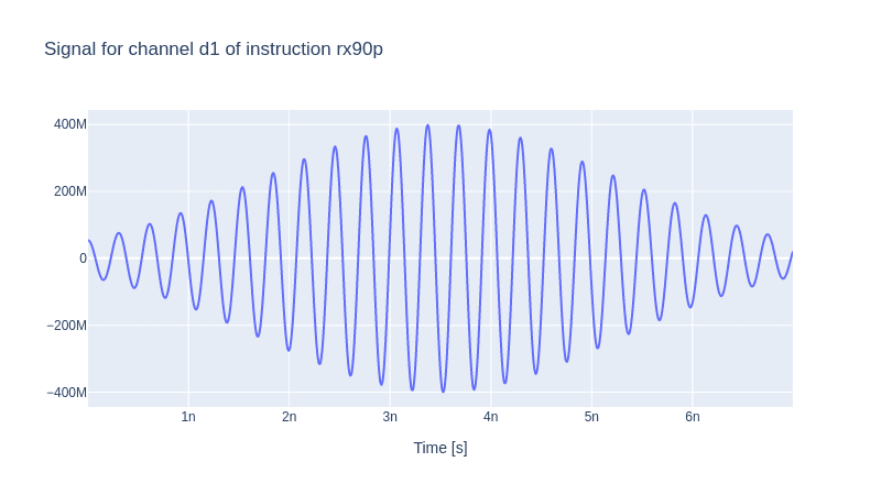
One can check the profile of the pulse by calling the generator.draw method.

generator.draw(instr=rx90p, resolution=sim_res)

2.3 Mapping the Parameters and Instantiating the Experiment

Hitherto, we have created our unimon and the pulse that carries our desired instruction set (gate). We have to specify how our Model and the Generator are mapped to the gate instruction we have just declared.

parameter_map = ParameterMap(
    instructions=[rx90p], model=model, generator=generator
)

simulation = Experiment(pmap=parameter_map, sim_res=sim_res)

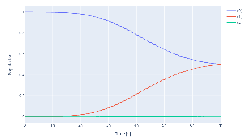
We can check the dynamics of our system under the action of our gate, namely rx90p, which should rotate the state of our unimon along the x-axis by 90 degrees yielding an equally split population between the states $\ket 0$ and $\ket 1$ .

# set the initial state to |0>
initial_state = model.get_state_of_label((0,))

# define the sequence of instructions under which
# the evolution takes place, in this case only the
# single struction rx90p
sequences = [rx90p.get_key()]

# compute the propagators and draw the dynamics
simulation.compute_propagators()
simulation.draw_dynamics(sequence=sequences, state=initial_state)

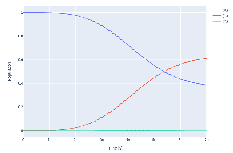
The fidelity of the gate is obviously low, as one sees in the figure above since the population does not get split between $\ket 0$ and $\ket 1$ . In the next step, we optimise our pulse to enhance the fidelity score of our gate.

2.4 Single-Qubit Gate Optimal Control

For an optimal control problem, one has to specify the score function and the subspace in which our goal function must get optimised.

log_dir = os.path.join(tempfile.TemporaryDirectory().name, "qruiselogs")

opt = OptimalControl(
    dir_path=log_dir,           # path to the logging directory
    fid_func=unitary_infid_set, # the fidelity function in this case unitary infidelity function
    fid_subspace=["Unimon"],    # the subspace in which the fidelity function must get optimised
    pmap=parameter_map,
    algorithm=lbfgs,            # optimisation algorithm
    options={"maxfun": 20},
    run_name="better_RX90",     # name to distinguish our logging records with
    logger=[PlotLineChart()],
)

# set the set of gates to be optimised
# in our case sequence = [rx90p.get_key()]
simulation.set_opt_gates(sequences)

# set the Experiment as the context of
# our optimisation problem
opt.set_exp(simulation)

Then, we specify the pulse parameters needed to be optimised

gateset_opt_map = [
    [
        (rx90p.get_key(), "d1", "gauss", "amp"),
    ],
    [
        (rx90p.get_key(), "d1", "gauss", "delta"),
    ],
    [
        (rx90p.get_key(), "d1", "gauss", "freq_offset"),
    ],
    [
        (rx90p.get_key(), "d1", "carrier", "freq"),

    ],
    [
        (rx90p.get_key(), "d1", "carrier", "framechange"),
    ],
]

parameter_map.set_opt_map(gateset_opt_map)

We can check the initial value of these parameters before the optimisation.

parameter_map.print_parameters()

rx90p[0]-d1-gauss-amp                 : 400.000 mV

rx90p[0]-d1-gauss-delta               : -1.000

rx90p[0]-d1-gauss-freq_offset         : -50.500 MHz 2pi

rx90p[0]-d1-carrier-freq              : 3.330 GHz 2pi

rx90p[0]-d1-carrier-framechange       : 0.000 rad

And finally optimising our pulse

opt.optimize_controls()

We can check the dynamics of the system after the optimisation by evolving the system under the action of the newly optimised pulse.

initial_state = model.get_state_of_label((0,))
simulation.compute_propagators()
simulation.draw_dynamics(sequence=sequences, state=initial_state)

And observe that indeed our gate performs RX90 rotation.

Compare the parameters of the optimised pulse to the unoptimised pulse.

parameter_map.print_parameters()

rx90p[0]-d1-gauss-amp                 : 349.194 mV

rx90p[0]-d1-gauss-delta               : -1.000

rx90p[0]-d1-gauss-freq_offset         : -50.498 MHz 2pi

rx90p[0]-d1-carrier-freq              : 3.333 GHz 2pi

rx90p[0]-d1-carrier-framechange       : -44.182 µrad

Obviously, it is nice to check the fidelity score as well

print(f" Fidelity: {(1 - opt.current_best_goal) * 100 : 4f}%")

Fidelity:  99.998390%

Of course, the trailing decimals could differ in different optimisation runs, but we have reached the 99.99% fidelity for our gate of interest.

2.5 Entangling two Unimons

2.5.1 The Hamiltonian

Unimons are capacitively coupled, similar to transmons, and use a cross-resonance scheme for entanglement. The schematic of such a coupling is demonstrated in the following diagram

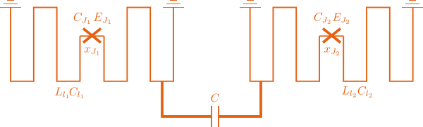
The Hamiltonian of the system at the sweet spot $\Phi_{\rm diff}= \Phi_0/2$ is given by the following expression

$\begin{aligned} \hat{H}_m = \sum_{i=1}^2 \Big[4E_{C,m}^i{\hat{n}_m^i}^2 + \frac{1}{2}E_{L,m}^i{\hat{\varphi}_m^i}^2 + E_J^i\cos(\hat{\varphi}_m^i)\Big] + E_c\hat{n}_m^1\hat{n}_m^2, \end{aligned}$

where the summation corresponds to the single Unimon Hamiltonians, and the last term is the coupling Hamiltonian between the two qubits.

Let's define a second unimon as the target qubit with a slightly different set of characteristics with respect to the previously created unimon, which we refer to as the control qubit.

# Target Unimon
unimon2_params ={
    "length": Quantity(
        value=4.0e-3, min_val=3.9e-3,
        max_val=4.1e-3, unit="m"),
    "capacitance_den": Quantity(
        value=83.2e-12, min_val=80e-12,
        max_val=86e-12, unit="F"),
    "inductance_den": Quantity(
        value=0.833e-6, min_val=0.80e-6,
        max_val=0.86e-6, unit="H/m"),
    "flux_diff": Quantity(
        value=Phi_0 / 2.0, min_val=Phi_0 * 0.48,
        max_val=Phi_0 * 0.55, unit="Wb"),
    "jj_inductance": Quantity(
        value=8.61e-9, min_val=8.5e-9,
        max_val=8.7e-9, unit="H"),
    "jj_capacitance": Quantity(
        value=1.39e-15, min_val=1.3e-15,
        max_val=1.5e-15, unit="F"),
    "jj_loc": Quantity(
        value=0.0, min_val=-0.1e-3,
        max_val=0.1e-3, unit="m")
}

q2 = Unimon(
    name="Unimon2", desc="Target Unimon",
    hilbert_dim=hilbert_dim, params=unimon2_params
)

And similarly, we assign a drive to our newly initialised target qubit

drive2 = components.Drive(
    name="d2",
    desc="Drive 2",
    comment="Drive line 2 on qubit 2",
    connected=["Unimon2"],
    hamiltonian_func=hamiltonians.x_drive,
)

Now we need to specify the coupling strength between the two unimons. The coupling strength $g_{01}$ is given by

$\begin{aligned} g_{01} = -\frac{E_c}{2} \sqrt{\frac{\beta_1\beta_2}{\alpha_1\alpha_2}}, \end{aligned}$

with $\alpha_i = \sqrt{4E_{C,m}^i}$ and $\beta_i = \sqrt{(E_{L,m}^i - E_J^i)/2}$ . We can use the function get_coupling_strength from the unimon.utils to get the coupling strength. Bear in mind that the output of the function must be multiplied by the capacitive energy of the coupling capacitance.

EC = 5e6 * 2.0 * np.pi
g01 = get_coupling_strength(q1, q2) * EC
q1q2 = components.Coupling(
    name="Unimon1-Unimon2",
    desc="coupling",
    comment="Coupling qubit 1 to qubit 2",
    connected=["Unimon1", "Unimon2"],
    strength=Quantity(
        value=g01, unit="Hz 2pi"),
    hamiltonian_func=hamiltonians.int_XX,
)

We then build the model by adding the second (target) qubit and the coupling between the two.

model = Model(
    subsystems=[q1, q2],
    couplings=[drive1, drive2, q1q2],
    dressed=True,
    lindbladian=False,
    use_FR=True)

2.5.2 Pulse Generator

Subsequently, we build our Generator stack

generator = Generator(
    devices={
        "LO": devices.LO(name="lo"),
        "AWG": devices.AWG(name="awg", resolution=awg_res),
        "DigitalToAnalog": devices.DigitalToAnalog(name="dac"),
        "Mixer": devices.Mixer(name="mixer"),
        "VoltsToHertz": devices.VoltsToHertz(
            name="v_to_hz",
            V_to_Hz=Quantity(
                value=1e9, min_val=0.9e9,
                max_val=1.1e9, unit="Hz/V"),
        ),
        "ResponseFFT": devices.ResponseFFT(
            name="ResponseFFT",
            rise_time=Quantity(
                value=5e-9,  unit="s")
        )
    },
    chains={
        "d1": {
            "LO": [],
            "AWG": [],
            "DigitalToAnalog": ["AWG"],
            "ResponseFFT": ["DigitalToAnalog"],
            "Mixer": ["LO", "ResponseFFT"],
            "VoltsToHertz": ["Mixer"],
        },
        "d2": {
            "LO": [],
            "AWG": [],
            "DigitalToAnalog": ["AWG"],
            "ResponseFFT": ["DigitalToAnalog"],
            "Mixer": ["LO", "ResponseFFT"],
            "VoltsToHertz": ["Mixer"],
        }
    },
)

In the cross-resonance scheme, both unimons are driven by a pulse tuned at the Rabi frequency of the target qubit, i.e. the second unimon. Once the model is built, we can access the Rabi frequency of each unimon by calling Unimon.params["freq"]. The following code block declares the parameters necessary to identify our Gaussian envelopes and the local oscillators for each unimon.

sideband = 50e6
lo_freq = q2.params["freq"] / (2 * np.pi) + sideband # Frequency of the local oscillator
awg_res = 1e11                                       # AWG resolution
t_final_2Q = 50e-9                                   # Pulse duration
sim_res = 1e11                                       # Simulation resolution
amp = [0.04, 0.4]                                    # amplitude of the control and target qubit respectively

The Gaussian envelopes,

# Gaussian envelop parameters for the control Unimon
gauss_params_u1 = {
    "amp": Quantity(
        value=amp[0], min_val=0.01 * amp[0],
        max_val=5.0 * amp[0], unit="V"),
    "t_final": Quantity(
        value=t_final_2Q, min_val=0.5 * t_final_2Q,
        max_val=1.5 * t_final_2Q, unit="s"
    ),
    "sigma": Quantity(
        value=t_final_2Q / 4, min_val=t_final_2Q / 8,
        max_val=t_final_2Q / 2, unit="s"
    ),
    "xy_angle": Quantity(
        value=-164.440e-3, min_val=-0.5 * np.pi,
        max_val=2.5 * np.pi, unit="rad"
    ),
    "freq_offset": Quantity(
        value=-sideband - 0.5e6,
        min_val=-60 * 1e6,
        max_val=-40 * 1e6,
        unit="Hz 2pi",
    ),
    "delta": Quantity(
        value=-1, min_val=-5,
        max_val=3, unit=""),
}

# Gaussian envelope parameters for the target Unimon
gauss_params_u2 = {
    "amp": Quantity(
        value=amp[1], min_val=0.01 * amp[1],
        max_val=5.0 * amp[1], unit="V"),
    "t_final": Quantity(
        value=t_final_2Q, min_val=0.5 * t_final_2Q,
        max_val=1.5 * t_final_2Q, unit="s"
    ),
    "sigma": Quantity(
        value=t_final_2Q / 4, min_val=t_final_2Q / 8,
        max_val=t_final_2Q / 2, unit="s"
    ),
    "xy_angle": Quantity(
        value=0.0, min_val=-0.5 * np.pi,
        max_val=2.5 * np.pi, unit="rad"
    ),
    "freq_offset": Quantity(
        value=-sideband - 0.5e6,
        min_val=-60 * 1e6,
        max_val=-40 * 1e6,
        unit="Hz 2pi",
    ),
    "delta": Quantity(
        value=-1, min_val=-5,
        max_val=3, unit=""),
}

gauss_env_u1 = pulse.Envelope(
    name="gauss",
    desc="Gaussian comp for two-qubit gate (Control)",
    params=gauss_params_u1,
    shape=envelopes.gaussian_nonorm,
)

gauss_env_u2 = pulse.Envelope(
    name="gauss",
    desc="Gaussian comp for two-qubit gate (Target)",
    params=gauss_params_u2,
    shape=envelopes.gaussian_nonorm,
)

and the Carriers are declared in due course.

# Pulse carrier of the control Unimon
carr_2Q_u1 = pulse.Carrier(
    name="carrier",
    desc="Carrier on drive 1",
    params={
        "freq": Quantity(
            value=lo_freq,
            min_val=0.01 * lo_freq,
            max_val=1.5 * lo_freq,
            unit="Hz 2pi",
        ),
        "framechange": Quantity(value=-1.014, min_val=-np.pi, max_val=3 * np.pi, unit="rad"),
    },
)

# Pulse carrier of the target Unimon
carr_2Q_u2 = pulse.Carrier(
    name="carrier",
    desc="Carrier on drive 2",
    params={
        "freq": Quantity(
            value=lo_freq,
            min_val=0.01 * lo_freq,
            max_val=1.5 * lo_freq,
            unit="Hz 2pi",
        ),
        "framechange": Quantity(value=1.260, min_val=-np.pi, max_val=3 * np.pi, unit="rad"),
    },
)

2.5.3 The CNOT Gate

For the pulse instruction, we declare the well-know CNOT gate

# CNOT comtrolled by qubit 1
cnot12 = gates.Instruction(
    name="cx",
    targets=[0, 1],         # specifying the target qubit
    t_start=0.0,
    t_end=t_final_2Q,
    channels=["d1", "d2"],
    ideal=np.array(         # the ideal CNOT gate
        [[1, 0, 0, 0],
         [0, 1, 0, 0],
         [0, 0, 0, 1],
         [0, 0, 1, 0]])
        )
cnot12.add_component(gauss_env_u1, "d1")
cnot12.add_component(carr_2Q_u1, "d1")
cnot12.add_component(gauss_env_u2, "d2")
cnot12.add_component(carr_2Q_u2, "d2")
cnot12.comps["d1"]["carrier"].params["framechange"].set_value(
    (-sideband * t_final_2Q) * 2 * np.pi % (2 * np.pi)
)

2.5.4 Mapping the Parameters and Instantiating the Experiment

We finally specify the ParameterMap and instantiate our Experiment as we did previously

parameter_map = ParameterMap(
    instructions=[cnot12], model=model, generator=generator
)

simulation = Experiment(pmap=parameter_map)

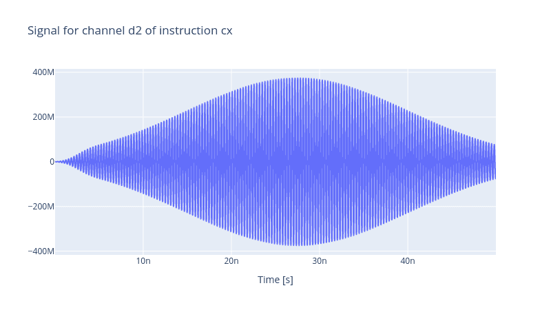
We can investigate the generated pulse for each channel

generator.draw(instr=cnot12, resolution=awg_res)

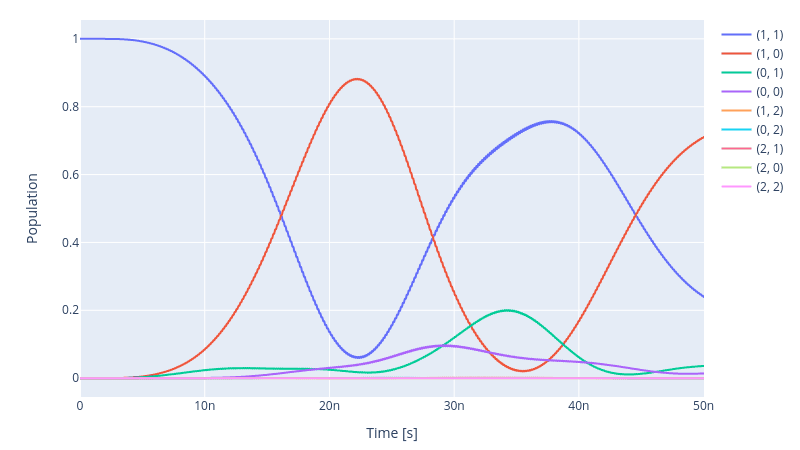
and as well the dynamics of the coupled unimon system under the action of the CNOT gate

initial_state = model.get_state_of_label((1, 1))
opt_gates = [cnot12.get_key()]
simulation.compute_propagators()
simulation.draw_dynamics(sequence=opt_gates, state=initial_state)

2.6 Two-Qubit Gate Optimal Control

The fidelity of our CNOT gate does not achieve our target goal where the final state must yield $|10\rangle$ . To optimise the pulse shape of the Gaussian envelopes of the channels, as we did in the previous section, we define an optimal control procedure as follows

log_dir = os.path.join(tempfile.TemporaryDirectory().name, "qruiselogs")

opt = OptimalControl(
    dir_path=log_dir,
    fid_func=unitary_infid_set,
    fid_subspace=["Unimon1", "Unimon2"],
    pmap=parameter_map,
    algorithm=lbfgs,
    options={"maxfun": 300},
    run_name="cnot12",
    logger=[PlotLineChart()],
)

simulation.set_opt_gates(opt_gates)
opt.set_exp(simulation)

We define the set of parameters that have to be optimised

gateset_opt_map = [
    [(cnot12.get_key(), "d1", "gauss", "amp")],
    [(cnot12.get_key(), "d1", "gauss", "freq_offset")],
    [(cnot12.get_key(), "d1", "gauss", "xy_angle")],
    [(cnot12.get_key(), "d1", "gauss", "delta")],
    [(cnot12.get_key(), "d1", "carrier", "framechange")],
    [(cnot12.get_key(), "d2", "gauss", "amp")],
    [(cnot12.get_key(), "d2", "gauss", "freq_offset")],
    [(cnot12.get_key(), "d2", "gauss", "xy_angle")],
    [(cnot12.get_key(), "d2", "gauss", "delta")],
    [(cnot12.get_key(), "d2", "carrier", "framechange")],
]

parameter_map.set_opt_map(gateset_opt_map)
parameter_map.print_parameters()

cx[0,1]-d1-gauss-amp                  : 40.000 mV
cx[0,1]-d1-gauss-freq_offset          : -50.500 MHz 2pi
cx[0,1]-d1-gauss-xy_angle             : -164.440 mrad
cx[0,1]-d1-gauss-delta                : -1.000
cx[0,1]-d1-carrier-framechange        : 3.142 rad
cx[0,1]-d2-gauss-amp                  : 400.000 mV
cx[0,1]-d2-gauss-freq_offset          : -50.500 MHz 2pi
cx[0,1]-d2-gauss-xy_angle             : -444.089 arad
cx[0,1]-d2-gauss-delta                : -1.000
cx[0,1]-d2-carrier-framechange        : 1.260 rad

After the optimisation we see that the evolution upon the action of the CNOT gate improves drastically.

initial_state = model.get_state_of_label((1, 1))

simulation.compute_propagators()
simulation.draw_dynamics(sequence=opt_gates, state=initial_state)

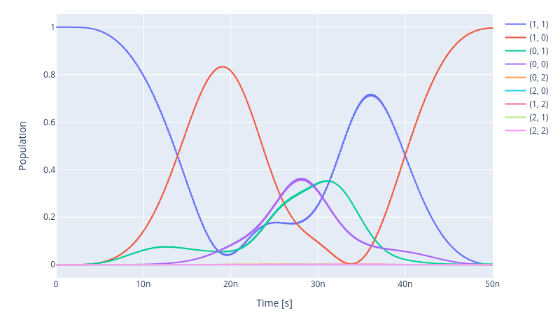
Yet, the fidelity is not promising

print(f" Fidelity: {(1 - opt.current_best_goal) * 100 : 4f}%")

Fidelity:  99.352600%

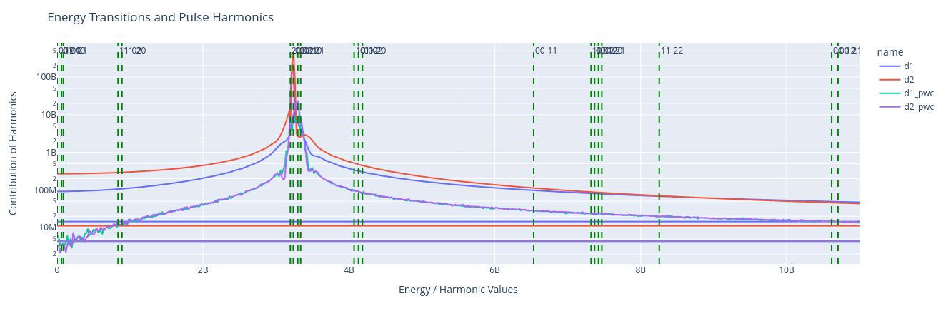
One can visualise the harmonics and how they overlap with the transition spectrum of the states. This enables one to investigate harmonics that cause spurious transitions and subsequently leads to leakage and low fidelity of the gate.

2.7 Two-stage optimal control

Within the framework discussed above, it is challenging to achieve a fidelity of 99.99%. This is due to the limitation we have regarding the dimension of the parameter space. Effectively, we can only vary in total three parameters of the Gaussian pulse, namely the amplitude, variance and polarization. This reduces the flexibility we can assert on our pulse shape. In what follows, we will show how we can take advantage of piece-wise linear pulses in a two-stage optimisation protocol to enhance fidelity.

What changes in this approach is the introduction of two piece-wise linear pulses, one for each channel

drive1 = components.Drive(
    name="d1",
    desc="Drive 1",
    comment="Drive line 1 on qubit 1",
    connected=["Unimon1"],
    hamiltonian_func=hamiltonians.x_drive,
)
drive2 = components.Drive(
    name="d2",
    desc="Drive 2",
    comment="Drive line 2 on qubit 2",
    connected=["Unimon2"],
    hamiltonian_func=hamiltonians.x_drive,
)

drive_pwl1 = components.Drive(
    name="d1_pwl",
    desc="pwl Drive 1",
    comment="Drive line 1 on qubit 1 for pwl pulse",
    connected=["Unimon1"],
    hamiltonian_func=hamiltonians.x_drive,
)
drive_pwl2 = components.Drive(
    name="d2_pwl",
    desc="pwl Drive 2",
    comment="Drive line 2 on qubit 2 for pwl pulse",
    connected=["Unimon2"],
    hamiltonian_func=hamiltonians.x_drive,
)

We add two more chains to our Generator to take into account these two drive lines

generator = Generator(
    devices={
        "LO": devices.LO(name="lo"),
        "AWG": devices.AWG(name="awg", resolution=awg_res),
        "DigitalToAnalog": devices.DigitalToAnalog(name="dac"),
        "Mixer": devices.Mixer(name="mixer"),
        "VoltsToHertz": devices.VoltsToHertz(
            name="v_to_hz",
            V_to_Hz=Quantity(
                value=1e9, min_val=0.9e9,
                max_val=1.1e9, unit="Hz/V"),
        ),
        "ResponseFFT": devices.ResponseFFT(
            name="ResponseFFT",
            rise_time=Quantity(
                value=5e-9,  unit="s")
        )
    },
    chains={
        "d1": {
            "LO": [],
            "AWG": [],
            "DigitalToAnalog": ["AWG"],
            "ResponseFFT": ["DigitalToAnalog"],
            "Mixer": ["LO", "ResponseFFT"],
            "VoltsToHertz": ["Mixer"],
        },
        "d1_pwl": {
            "LO": [],
            "AWG": [],
            "DigitalToAnalog": ["AWG"],
            "ResponseFFT": ["DigitalToAnalog"],
            "Mixer": ["LO", "ResponseFFT"],
            "VoltsToHertz": ["Mixer"],
        },
        "d2": {
            "LO": [],
            "AWG": [],
            "DigitalToAnalog": ["AWG"],
            "ResponseFFT": ["DigitalToAnalog"],
            "Mixer": ["LO", "ResponseFFT"],
            "VoltsToHertz": ["Mixer"],
        },
        "d2_pwl": {
            "LO": [],
            "AWG": [],
            "DigitalToAnalog": ["AWG"],
            "ResponseFFT": ["DigitalToAnalog"],
            "Mixer": ["LO", "ResponseFFT"],
            "VoltsToHertz": ["Mixer"],
        }
    },
)

It is worth mentioning that these two extra drives, namely drive_pwl1 and drive_pwl2, are not two separate drive lines. It will be elaborated soon that we let our mixer carry out the mixing of the Gaussian envelopes and the piece-wise linear (PWL) envelopes within a single carrier. But let's first proceed with defining our PWL envelopes

# number of pwl which is practically the
# total number simulation steps
slices = int(round(t_final_2Q * awg_res))
pwl_params_u1 = {
    # use small but nonzero initial values to try to avoid local minima and ensure non-zero grad
    "inphase": Quantity(
        value=(np.random.rand(slices)*2 -1.0)/100,
        min_val=-0.25, max_val=0.25, unit="V"
    ),
    "t_sampled": Quantity(
        value=np.linspace(0, t_final_2Q, slices + 1)[:-1] +\
              np.linspace(0, t_final_2Q, slices + 1)[1:],
        unit="s"),
    "t_final": Quantity(
        value=t_final_2Q, min_val=0.5 * t_final_2Q,
        max_val=1.5 * t_final_2Q, unit="s"
    )
}

pwl_params_u2 = {
    # use small but nonzero initial values to try to avoid local minima and ensure non-zero grad
    "inphase": Quantity(
        value=(np.random.rand(slices)*2 -1.0)/100,
        min_val=-0.25, max_val=0.25, unit="V"
    ),
    "t_sampled": Quantity(
        value=np.linspace(0, t_final_2Q, slices + 1)[:-1] +\
              np.linspace(0, t_final_2Q, slices + 1)[1:],
        unit="s"),
    "t_final": Quantity(
        value=t_final_2Q, min_val=0.5 * t_final_2Q, max_val=1.5 * t_final_2Q, unit="s"
    )
}

pwl_env_u1 = pulse.Envelope(
    name="pwl",
    desc="pwl envelope on d1_pwl",
    params=pwl_params_u1,
    shape=envelopes.pwl_shape_sampled_times,
)

pwl_env_u2 = pulse.Envelope(
    name="pwl",
    desc="pwl envelope on d2_pwl",
    params=pwl_params_u2,
    shape=envelopes.pwl_shape_sampled_times,
)

The Gaussian envelopes are the same as in the previous subsection as well as the carries. Now let us reintroduce our CNOT gate

# CNOT comtrolled by qubit 1
cnot12 = gates.Instruction(
    name="cx",
    targets=[0, 1],
    t_start=0.0,
    t_end=t_final_2Q,
    channels=["d1", "d2", "d1_pwl", "d2_pwl"],
    ideal=np.array([[1, 0, 0, 0], [0, 1, 0, 0], [0, 0, 0, 1], [0, 0, 1, 0]]),
)
cnot12.add_component(gauss_env_u1, "d1")
cnot12.add_component(carr_2Q_u1, "d1")

cnot12.add_component(pwl_env_u1, "d1_pwl")
cnot12.add_component(carr_2Q_u1, "d1_pwl")

cnot12.add_component(gauss_env_u2, "d2")
cnot12.add_component(carr_2Q_u2, "d2")

cnot12.add_component(pwl_env_u2, "d2_pwl")
cnot12.add_component(carr_2Q_u2, "d2_pwl")

cnot12.comps["d1"]["carrier"].params["framechange"].set_value(
    (-sideband * t_final_2Q) * 2 * np.pi % (2 * np.pi)
)

Now notice that the d1 and d1_pwl are both added to the same carrier. The same applies to the d2 and d2_pwl lines. Finally we can instantiate our ParameterMap and the Model

parameter_map = ParameterMap(
    instructions=[cnot12], model=model, generator=generator
)

simulation = Experiment(pmap=parameter_map)

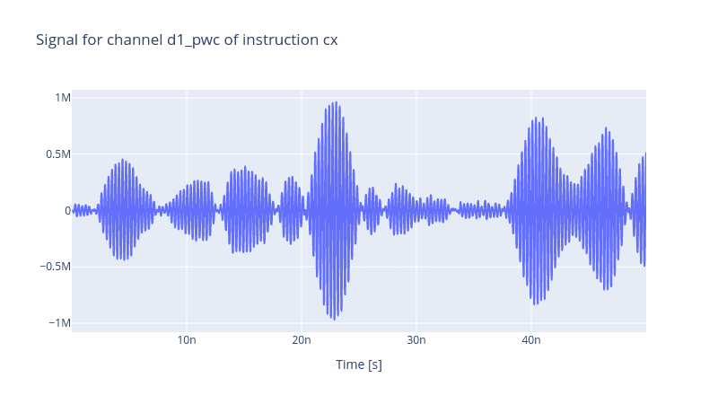
When we plot the pulses generated by our Generator, in addition to the two Gaussian pulses shown previously, one identifies two more PWL pulses present in d1_pwl and d2_pwl channels

2.7.1 Pulse Optimisation: Stage One

In the first stage, we optimise the parameters of our Gaussian envelopes. This eases up the next stage of the optimisation by providing it with a better initial guess. First, define the optimal control problem

opt = OptimalControl(
    dir_path=log_dir,
    fid_func=unitary_infid_set,
    fid_subspace=["Unimon1", "Unimon2"],
    pmap=parameter_map,
    algorithm=lbfgs,
    options=options_lbfgs,
    run_name="cnot12",
    logger=[PlotLineChart()],
)

simulation.set_opt_gates(opt_gates)
opt.set_exp(simulation)

and then set the optimal control map

gateset_opt_map = [
    [(cnot12.get_key(), "d1", "gauss", "amp")],
    [(cnot12.get_key(), "d1", "gauss", "freq_offset")],
    [(cnot12.get_key(), "d1", "gauss", "xy_angle")],
    [(cnot12.get_key(), "d1", "gauss", "delta")],
    [(cnot12.get_key(), "d1", "carrier", "framechange")],

    [(cnot12.get_key(), "d2", "gauss", "amp")],
    [(cnot12.get_key(), "d2", "gauss", "freq_offset")],
    [(cnot12.get_key(), "d2", "gauss", "xy_angle")],
    [(cnot12.get_key(), "d2", "gauss", "delta")],
    [(cnot12.get_key(), "d2", "carrier", "framechange")],
]

parameter_map.set_opt_map(gateset_opt_map)

After optimisation, we get a similar result as demonstrated in the previous subsection. But then we define the parameter map of the second stage of the optimisation.

gateset_opt_map = [
    [(cnot12.get_key(), "d1", "gauss", "amp")],
    [(cnot12.get_key(), "d1", "gauss", "freq_offset")],
    [(cnot12.get_key(), "d1", "gauss", "xy_angle")],
    [(cnot12.get_key(), "d1", "gauss", "delta")],
    [(cnot12.get_key(), "d1", "carrier", "framechange")],

    [(cnot12.get_key(), "d2", "gauss", "amp")],
    [(cnot12.get_key(), "d2", "gauss", "freq_offset")],
    [(cnot12.get_key(), "d2", "gauss", "xy_angle")],
    [(cnot12.get_key(), "d2", "gauss", "delta")],
    [(cnot12.get_key(), "d2", "carrier", "framechange")],

    [(cnot12.get_key(), "d1_pwl", "pwl", "inphase")],
    [(cnot12.get_key(), "d2_pwl", "pwl", "inphase")]
]

parameter_map.set_opt_map(gateset_opt_map)

Now observe that we have added the parameters of the PWL envelopes for the optimisation. We run the optimisation. At this stage, expect the optimisation to take longer as we have expanded the dimension of our parameter space significantly. After the optimisation is done, we can check the evolution of the system after applying the optimised CNOT gate

initial_state = model.get_state_of_label((1, 1))

simulation.compute_propagators()
simulation.draw_dynamics(sequence=opt_gates, state=initial_state)

At first glance, this figure looks just like the same as the one we presented in the single-stage optimisation protocol. But a closer inspection shows that the fidelity has improved noticeably.

print(f" Fidelity: {(1 - opt.current_best_goal) * 100 : 4f}%")

Fidelity:  99.996482%

And compare the harmonics that contribute to the dynamics to the one shown previously in the previous section when PWL lines were absent.

References

Share this post

Share on X

Share on LinkedIn

Stay Informed with Our Newsletter

Subscribe to our newsletter to get the latest updates on our products and services.

References

- [1]. Hyyppä, Eric, Suman Kundu, Chun Fai Chan, András Gunyhó, Juho Hotari, David Janzso, Kristinn Juliusson et al. "Unimon qubit." Nature Communications 13, no. 1 (2022): 6895.
- [2]. Bourassa, J., F. Beaudoin, Jay M. Gambetta, and A. Blais. "Josephson-junction-embedded transmission-line resonators: From Kerr medium to in-line transmon." Physical Review A 86, no. 1 (2012): 013814.
- [3]. Krantz, Philip, Morten Kjaergaard, Fei Yan, Terry P. Orlando, Simon Gustavsson, and William D. Oliver. "A quantum engineer's guide to superconducting qubits." Applied physics reviews 6, no. 2 (2019): 021318.