Advanced Modelling of the Control Stack with Response Functions

Knowing all the characteristics of an electronic device is impractical. With many other factors at play affecting the quality of the desired pulse, such as the bandwidth of the wires through which the pulse arrives at the target qubit, temperature, background noise and many other factors influencing the output pulse, the complexity of the modelling grows and hence is intractable to model. Due to this, electronic devices are often characterised by their response function. It indicates how the electronic device's response to a change in the input signal alters the output signal accordingly. The response function is defined theoretically in the Laplace space as

$H(s) = \frac{Y(s)}{X(s)},$

where $Y(s)$ and $X(s)$ are the output and input signals respectively. In the Qruise toolset, the user can define the response function of a given device. This powerful tool yet imposes some limitations. Although one can counteract the effect of the response function, the origin of sources that lead to such dynamics remains unknown. Therefore, it is impossible to investigate how strongly or weakly they affect the fidelity of a given operation.

Our implementation of the response function is via a ResponseFunc device object. It is a pseudo-device like the DigitalToAnalog or RiseTime device, and it only has a meaning when it appears in the control stack in juxtaposition with a generic device such as an AWG.

A response function $H(s)$ expressed as

$H(s) = \frac{\sum_{i=0}^n b_i s^i}{\sum_{j=0}^m a_j s^j}$

is uniquely identified by the coefficients of the nominator i.e. $\{b_i\}_{i=0}^n$ and the coefficients of the denominator i.e. $\{a_j\}_{j=0}^m$. These two lists of coefficients are sufficient to characterise and instantiate a ResponseFunc device. Initially, it is important to define the drive line.

from qruise.toolset.libraries import components, hamiltonians

flux_line = components.Drive(
    name="flux_line",
    connected=["Qubit_0"],
    hamiltonian_func=hamiltonians.x_drive,
)

We assume a control stack consisting of only a single AWG component with its DAC component. For the time being, we avoid adding the response function of the AWG to be able to distinguish its effect.

from qruise.toolset.objects import Quantity as Qt
from qruise.toolset.generator.devices import OEMAWG, DigitalToAnalog, VoltsToHertz

awg_params = {
    "name": "AWG",  # given name of the device
    "sim_time": 20e-9,  # 20ns (pulse duration)
    "samp_rate": int(2.4e9),  # 2.4 GHz sample rate
    "waveform_granularity": 8,  # granularity of the AWG device
    "min_waveform_len": 16,  # shortest (in number of samples) waveform AWG can produce
}


dac_params = {
    "nob": 16,  # number of bits
    "min_range": -2.5,  # minimum range of the output voltage
    "max_range": 2.5,  # maximum range of the output voltage
}

stack_devices = {
    "AWG": OEMAWG(**awg_params),
    "DAC": DigitalToAnalog(name="DAC", **dac_params),
    "V2Hz": VoltsToHertz(
        name="V2Hz", V_to_Hz=Qt(value=1.0, unit="V/Hz")
    ),
}

stack_chain = {"flux_line": {"AWG": [], "DAC": ["AWG"], "V2Hz": ["DAC"]}}

Assume a Gaussian envelope

from qruise.toolset.signal import pulse

t_gate = stack_devices["AWG"].sim_time
gauss_params = {
    "amp": Qt(
        value=1.0, min_val=-2.5, max_val=2.5, unit="V"
    ),  # maximum amplitude of the Gaussian envelope
    "t_final": Qt(
        value=t_gate, unit="s"
    ),  # the final time at which the envelope is set to zero
    "sigma": Qt(value=0.25 * t_gate, unit="s"),  # the variance of the Gaussian envelope
}
gauss_env = pulse.Envelope(
    name="gauss_env",
    params=gauss_params,
    shape=pulse.envelopes.gaussian_nonorm,  # here we specify the shape of the envelope
)

with an identity gate operation for the instruction.

from qruise.toolset.signal import gates
from qruise.toolset.libraries import constants

instr = gates.Instruction(
    name="id",  # name of the instruction
    t_end=t_gate,  # duration of the instruction (pulse duration)
    channels=["flux_line"],  # to which channel the instruction (pulse) is applied
    targets=[0],  # the index of the target qubit (not relevant but mandatory)
    ideal=constants.Id,
)

instr.add_component(comp=gauss_env, chan="flux_line")

Lastly, declare the Generator and produce the output pulse.

from qruise.toolset.generator.generator import Generator

generator = Generator(devices=stack_devices, chains=stack_chain)
generator.draw(instr=instr, resolution=1e11)

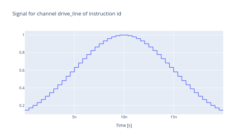
This profile is expected from a Gaussian envelope generated by an AWG with its DAC component. Notice that the pulse reaches its maximum amplitude value of 1.0V, and the dents are pretty sharp. Such behaviour was also demonstrated in our blog post regarding the effect of the DAC component.

Let us use the scipy.signal.butter filter to get the polynomial coefficients of a low-pass Butterworth filter. Although those coefficients can be passed by the user's input independently, the usage of the scipy library is solely for ease of demonstration.

from scipy import signal

half_power_freq = 300e6  # -3dB frequency of the Butterworth filter
num_poly, den_poly = signal.butter(
    N=4, Wn=half_power_freq, btype="low", fs=stack_devices["AWG"].samp_rate
)  # Butterworth filter of order N=4

Now we are ready to add a ResponseFunc to the control stack by passing the list of the coefficients.

from qruise.toolset.generator.devices import ResponseFunc

stack_devices["RespFunc"] = ResponseFunc(
    name="RespFunc", num_poly=num_poly, den_poly=den_poly
)
stack_chain = {
    "flux_line": {"AWG": [], "DAC": ["AWG"], "RespFunc": ["DAC"], "V2Hz": ["RespFunc"]}
}

generator = Generator(devices=stack_devices, chains=stack_chain)

And draw the output signal.

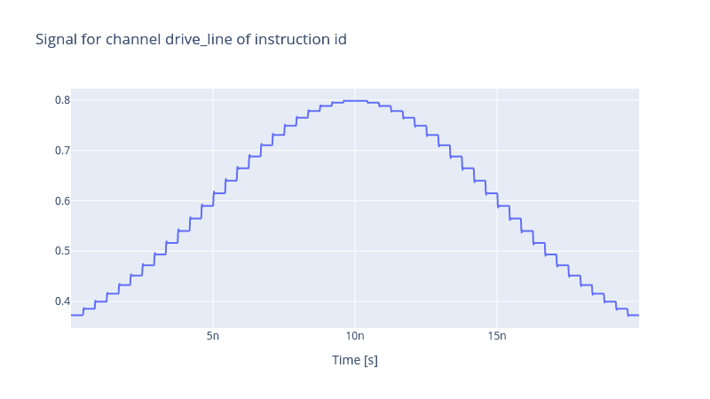
generator.draw(instr=instr, resolution=1e11, line_shape="spline")

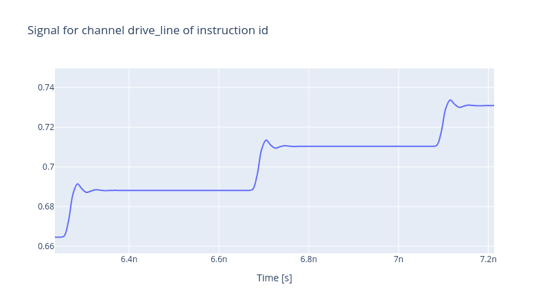
If one zooms in on the edges of the dents, the ringing, overshooting and relaxation effects due to the response function become clearer.