So far, we have spent a fair amount of time on properties of arbitrary waveform generators and discussed how we can tune, for instance, the resonant frequency of a qubit via a flux line. We also addressed two pseudo-devices namely RiseTime and DigitalToAnalog. Nonetheless, we are missing an essential component that enables us to drive a target qubit by performing actual gate operation via a finely tailored pulse.

The local oscillator is that missing component. It operates at way higher frequency ranges than AWGs, and together they provide a powerful tool to control the output signal that suits the purpose of driving a qubit at the resonant frequency. Yet, they are inherently noisy like any other electronic device. The two main sources of noise that affect the output of a local oscillator are amplitude noise and phase noise. Here, we demonstrate how easily we can introduce a noisy local oscillator in the control stack. Initially, we create a noiseless local oscillator, first to show how in the Qruise toolset we need a carrier in our instruction that encodes the information of the local oscillator. Then we introduce the amplitude and phase noises separately to show how each one of these noise sources distorts the final output pulse.

This time, contrary to the case when we had only a single AWG in our control stack, we define a drive line

from qruise.toolset.libraries import components, hamiltonians

drive_line = components.Drive(
    name="drive_line",
    connected=["Qubit_0"],
    hamiltonian_func=hamiltonians.x_drive,
)

Then we define the control stack and the chain. We want to have only a local oscillator in the stack which receives two parameters, the phase_noise and the amp_noise. As said before, we intend to have a noiseless local oscillator initially. Thus we set them both to None for the time being.

from qruise.toolset.objects import Quantity as Qt
from qruise.toolset.generator.devices import OEMLO, VoltsToHertz

lo_params = {
    "phase_noise": None,
    "amp_noise": None,
}


stack_devices = {
    "LO": OEMLO(name="Local oscillator", **lo_params),
    "V2Hz": VoltsToHertz(
        name="V2Hz", V_to_Hz=Qt(value=1.0, unit="V/Hz")
    ),
}

stack_chain = {"drive_line": {"LO": [], "V2Hz": ["LO"]}}

A sharp observer notices that we have not yet passed the frequency of the local oscillator. In the Qruise toolset, the information of the local oscillator is embodied in a Carrier object. This carrier is then added to the Instruction establishing the connection between the local oscillator and the instruction delivered to the target qubit.

from qruise.toolset.signal import pulse

lo_freq = 5.0e6

carr_params = {
    "freq": Qt(
        value=lo_freq, min_val=0.9 * lo_freq, max_val=1.1 * lo_freq, unit="Hz 2pi"
    ),
}

carr = pulse.Carrier(name="carrier", params=carr_params)

For simplicity, as always, let us choose an identity instruction and add the previously defined carrier component to it.

from qruise.toolset.signal import gates
from qruise.toolset.libraries import constants

t_gate = 1e-6
instr = gates.Instruction(
    name="id",  # name of the instruction
    t_end=t_gate,  # duration of the instruction (pulse duration)
    channels=["drive_line"],  # to which channel the instruction (pulse) is applied
    targets=[0],  # the index of the target qubit (not relevant but mandatory)
    ideal=constants.Id,
)

instr.add_component(carr, "drive_line")

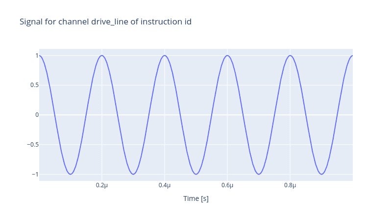
And finally, declare the Genarator,

from qruise.toolset.generator.generator import Generator

generator = Generator(devices=stack_devices, chains=stack_chain)
generator.draw(instr=instr, resolution=1e9)

The pulse above, as expected, is pretty smooth. Let us add an amplitude noise to it. We can conceive it as an Orstein-Uhlenbeck process where the amplitude deviates slightly from its actual value and then returns to its stationary value. Qruise toolset has a variety of noise processes, such as the white Gaussian noise, Ornstein-Uhlenbeck noise, the class of coloured noises, etc.

The noise processes themselves have a set of parameters. For instance, the Ornstein-Uhlenbeck process takes two parameters $\theta$, which is called the inverse of the mean reversion time, and $\sigma$, which is the strength of the fluctuations of the white noise. The larger the first value, the faster the return to the stationary value is, and the larger the latter, the stronger the fluctuations will be. Therefore, it is crucial to fine-tune these parameters to replicate the same noise profile a real local oscillator exhibits.

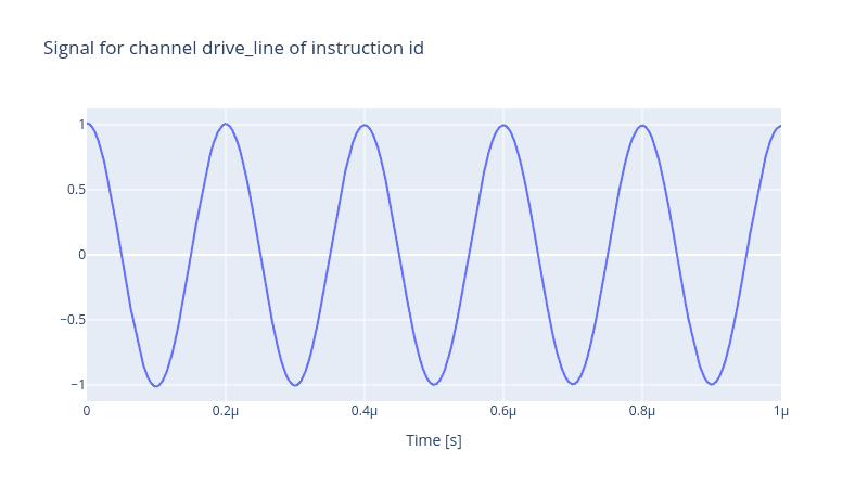
Let us now add an amplitude noise to our local oscillator and add it to the control stack and then generate the output signal

from qruise.toolset.libraries.noise.noises import ornstein_uhlenbeck_noise

lo_params = {
    "phase_noise": None,
    "amp_noise": (
        ornstein_uhlenbeck_noise,
        {"theta": 5e-5 / t_gate, "sigma": 1e-2},
    ),
}

stack_devices["LO"] = OEMLO(name="Local oscillator", **lo_params)

generator = Generator(devices=stack_devices, chains=stack_chain)
generator.draw(instr=instr, resolution=1e11)

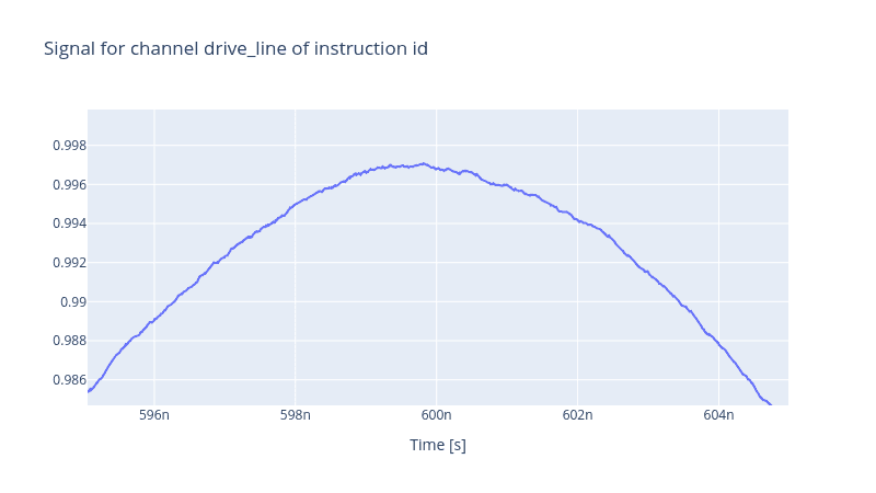
If we zoom in at the troughs and ridges, the effect of the noise becomes apparent. Also, since this is a random process, every time we generate a signal, the output will be different.

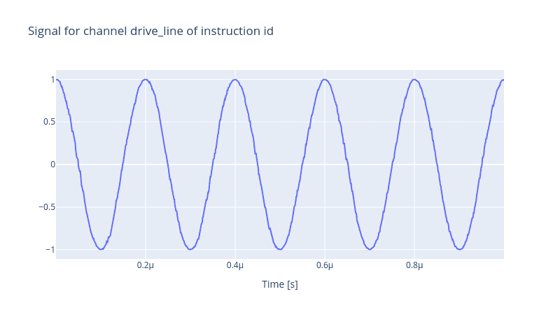
The phase noise is another source of imperfection. Often, the phase noise exhibits a $1/f$ power spectral density profile for low-range frequencies suggesting a coloured noise process. In the Qruise toolset, the coloured_noise function realises $1/f^\alpha$ processes for a real-valued $\alpha$ variable. It also has an extra parameter called q, which tunes the strength of the noise.

from qruise.toolset.libraries.noise.noises import coloured_noise

lo_params = {
    "phase_noise": (coloured_noise, {"alpha": -0.5, "q": 1e3}),
    "amp_noise": None,
}

stack_devices["LO"] = OEMLO(name="Local oscillator", **lo_params)

In the cell above, we have declared a pink noise which has $\alpha=-0.5$ indicating $(1/f)^{2\alpha} = 1/f$. Note that the value of alpha is half of the value one observes in the power spectral density, simply due to the fact that the power spectral density is the second power of the noise process. Now let us generate the pulse

generator = Generator(devices=stack_devices, chains=stack_chain)
generator.draw(instr=instr, resolution=1e9)