In the last century, the advent of magnetic resonance imaging (MRI) transformed medical diagnostics. Unlike methods that use ionizing radiation, MRI utilizes magnetic fields and radio waves, offering a safer imaging alternative.

The core principle of MRI is leveraging large magnetic fields to influence the precession frequencies of hydrogen nuclei in the body. The polarization (P) in this context can be described by the formula:

where γ is the gyromagnetic ratio, h is Planck’s constant, B0 is the magnetic field strength, kB is Boltzmann's constant, and T is the temperature.

This leads to the magnetization (M) being expressed as:

where N represents the number of spins. The quality of the MRI signal is directly proportional to the magnetization, and so the higher the magnetization, the better the image quality. So to increase the magnetisation of our sample we can try manipulating N, B0, or T. However, altering these variables within the constraints of human physiology presents a challenge.

Increasing the magnetisation is important especially in the field of metabolic imaging which has received a lot of interest in the last few years. The ability to monitor in real time how different diseases metabolise molecules could lead to huge breakthroughs in their treatment. To do this monitoring we want to be able to monitor the 13C signal during a metabolic process. Thus we need to increase the magnetisation signal somehow, and hyperpolarization techniques offer a neat solution to this. Signal enhancements by factors of between 10^4 to 10^5, can be expected, with very few changes required to existing MRI hardware.

Hyperpolarization Techniques

Dynamic nuclear polarization (DNP) has been a frontrunner, utilizing polarized electron spins to transfer polarization to nuclear spins, albeit with hurdles including high costs and operational intricacies.

A promising alternative is para-hydrogen induced polarization (PHIP), and notably, the PHIPSAH variant introduced by Francesca Reineri in 2015. Here, an unsaturated precursor molecule undergoes hydrogenation with para-hydrogen, facilitating hyperpolarization. This process culminates in transferring this enhanced polarization to 13C magnetization, broadening the horizons for detailed metabolic imaging. This method is simple, the experimental setups work at room temperature and are typically small and inexpensive to assemble. Commercial para-hydrogen generators are available, and so the barrier to entry is low.

We'll now demonstrate how to do this in Qruise!

Simple Qruise Simulations

We can start by creating the necessary spin objects:

tpi = 2 * np.pi
γh = 42.577 * tpi
γc = 10.708 * tpi

# carbon is nr 1, protons 2, 3
h1 = Spin("H1", hilbert_dim=2, params={"gamma": γh})
h2 = Spin("H2", hilbert_dim=2, params={"gamma": γh})
c = Spin("C", hilbert_dim=2, params={"gamma": γc})

then we describe the coupling between the spins, in this case its a j_coupling:

J12_val = Quantity(6.6 * tpi)
J13_val = Quantity(3.2 * tpi)
J23_val = Quantity(15.7 * tpi)

# J couplings between the spins
J12 = Coupling(
    name="J12", strength=J12_val, hamiltonian_func=j_coupling, connected=["C", "H1"]
)
J13 = Coupling(
    name="J13", strength=J13_val, hamiltonian_func=j_coupling, connected=["C", "H2"]
)
J23 = Coupling(
    name="J23", strength=J23_val, hamiltonian_func=j_coupling, connected=["H1", "H2"]
)

We also create some drives, which capture how the spin system will interact with an applied magnetic field, in this case, the magnetic field will simply interact with the Z component of the spin:

H1d = DriveSpinScaled(
    name="H1_drive", hamiltonian_func=offset, connected=["H1"], params={"alpha": γh}
)
H2d = DriveSpinScaled(
    name="H2_drive", hamiltonian_func=offset, connected=["H2"], params={"alpha": γh}
)
Cd = DriveSpinScaled(
    name="C_drive", hamiltonian_func=offset, connected=["C"], params={"alpha": γc}
)

Finally, we set up the Qruise model:

model = Model(
    subsystems=[c, h1, h2],
    couplings=[J12, J13, J23, H1d, H2d, Cd],
    dressed=False,
    use_FR=False,
)

Now we have our molecule set up, it's time to mimic the hydrogenation step. The model we use in Qruise is actually the already hydrogenated fumarate (not the precursor) so we simulate a fake hydrogenation step at $4\mu \text{T}$ for $15\text{s}$ (as in the experiment) which washes away some coherences.

This is simple to model in Qruise:

H0, Ht = model.get_Hamiltonians() # get the drift and control Hamiltonians

# define the field at which we hydrogenate
drive = 4.0  # uT
# define the duration of the hydrogenation (we use a list here so we get the intermediate states)
t_list = np.linspace(0, 15, 100)

# then define the Hamiltonians and their associated drives
H = [
    H0,
    [Ht["H1_drive"] * γh, drive],
    [Ht["H2_drive"] * γh, drive],
    [Ht["C_drive"] * γc, drive],
]
# finally we collect everything together into a Context object in Qruise, this captures all of the information necessary to describe the dynamics
ctx = DummyContext(H, t_list)

Then we simply propagate our system, save the intermediate states, and then average the density matrix across all the timesteps, washing out the coherences, similar to hydrogenation:

U = propagate(ctx, accum=True)
init_state = get_initial_state_generic([c, h1, h2], [1, 2])

all_states = []
for u in U:
    all_states.append(u @ init_state @ u.T.conj())

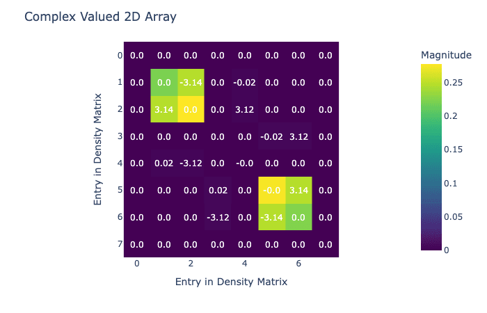
avg_state = np.mean(all_states, axis=0)
visualize_density_matrix(avg_state)

Now we have our density matrix after hydrogenation, it's time to do the field sweep that transfers magnetization. In this case we're going to do a simple linear sweep, but in Qruise it would be easy to replace this with an optimized sweep.

n_pts = 100
duration = 5.0
sweep_range = np.array([50 / 1000, 1])  # 0 to 1uT
x_lin = np.linspace(0, duration, n_pts)
sweep = sweep_range[0] + x_lin / duration * (sweep_range[1] - sweep_range[0])

# the same as before we create our context object, notice here we pass in a vector of the drives, which will be used to define the Hamiltonian at every point in time:
H = [
    H0,
    [Ht["H1_drive"] * γh, sweep],
    [Ht["H2_drive"] * γh, sweep],
    [Ht["C_drive"] * γc, sweep],
]

ctx = DummyContext(H, x_lin)

Then we can use the same propagate command to solve the problem:

all_states = []
U = propagate(ctx, accum=True)
for u in U:
    all_states.append(u @ avg_state @ u.T.conj())

And to visualise the growth of the polarization we trace out the Carbon spin $\sigma_Z$ value:

czs = embed([c, c, c], 0, PAULIS["Z"]) / 2
cz = [np.real(np.trace(czs @ i)) for i in all_states]

fig = plot_dynamics(
    np.array(cz).reshape(1, len(cz)),
    sim_res=1,
    state_labels=["SZ"],
    best_scored=-1,
    downsampling_threshold=-1,
)
fig.update_xaxes(title="Slice index")
fig.update_yaxes(title="Carbon SZ Value")

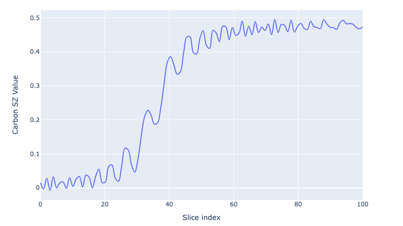
We go from 0 carbon polarization to a fully polarized Carbon spin (or as close as we can get after the coherences are washed away!).