We are surrounded by digital devices, mobile phones, computers, audio players, and many other devices that use binary representations of information to process data and convert them to analogue signals. At the heart of this technology is the Digital Analogue Converter (DAC) that bridges the worlds of binary and continuous representation of signals. Think of the Riemann integral, where a continuous curve is broken into discrete rectangular pieces to approximate the area under the curve. The finer the discretised intervals are, the more accurate the area under the curve is. Similarly, a DAC estimates the amplitude of a continuous curve using discrete values. Every DAC is characterised by its number of bits (NOB) which indicates how precisely it can approximate continuous values. For instance, if a DAC has 4 NOBs and the range of its operational voltage is from -2.5V to 2.5V, the digital values of the voltage are 16 values in total i.e. {-2.5V, -2.1875V, -1.875V, ..., 1.5625V, 1.875V, 2.1875V} with the increment of 0.3125V. It is worth mentioning that, in practice, DAC devices have an effective number of bits (ENOB) due to noise and quantisation errors, a number always smaller than NOB.

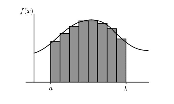
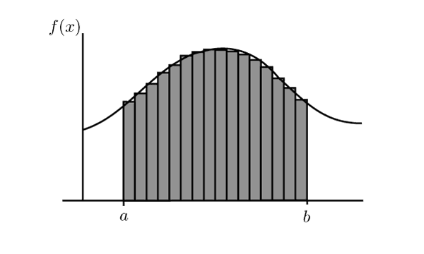
Riemann Integral, discretisation of a contiuous curve. The finer the intervals are, the better the area under the curve is approximated. The same idea applies to DACs, the higher the NOB, the finer the representation of a continuous analogue signal would be.

In our previous blog, we discussed some of the features of AWGs modelled in the Qruise toolset. Yet, an AWG is inherently a digital device and thus has a DAC component. To replicate this behaviour, one can use the DigitalToAnalog device in the Qruise toolset and specify the NOB of the device. Since DigitalToAnalog is a pseudo-device as it is not autonomous by itself but rather comes in combination with other generic electronic devices such as an AWG, the content presented here can be considered as a natural extension to a more realistic AWG device. Let us assume that our AWG operates between -2.5V and 2.5V and has 16 NOB.

First, it is essential to declare the flux (drive) line first.

from qruise.toolset.libraries import components, hamiltonians

drive_line = components.Drive(
    name="flux_line",
    connected=["Qubit_0"],
    hamiltonian_func=hamiltonians.x_drive,
)

Then define the parameters of the AWG and its DAC component, construct the control stack and declare the connectivity of the components.

from qruise.toolset.objects import Quantity as Qt
from qruise.toolset.generator.devices import OEMAWG, DigitalToAnalog, VoltsToHertz

# simulation resolution, different than the AWG sampling rate
sim_res = 1e11

awg_params = {
    "name": "AWG",  # given name of the device
    "sim_time": 20e-9,  # 20ns (pulse duration)
    "samp_rate": int(2.4e9),  # 2.4 GHz sample rate
    "waveform_granularity": 8,  # granularity of the AWG device
    "min_waveform_len": 16,  # shortest (in number of samples) waveform AWG can produce
}


dac_params = {
    "nob": 16,  # number of bits
    "min_range": -2.5,  # minimum range of the output voltage
    "max_range": 2.5,  # maximum range of the output voltage
}


stack_devices = {
    "AWG": OEMAWG(**awg_params),
    "DAC": DigitalToAnalog(name="DAC", **dac_params),
    "V2Hz": VoltsToHertz(
        name="V2Hz", V_to_Hz=Qt(value=1.0, unit="V/Hz")
    ),
}

stack_chain = {"flux_line": {"AWG": [], "DAC": ["AWG"], "V2Hz": ["DAC"]}}

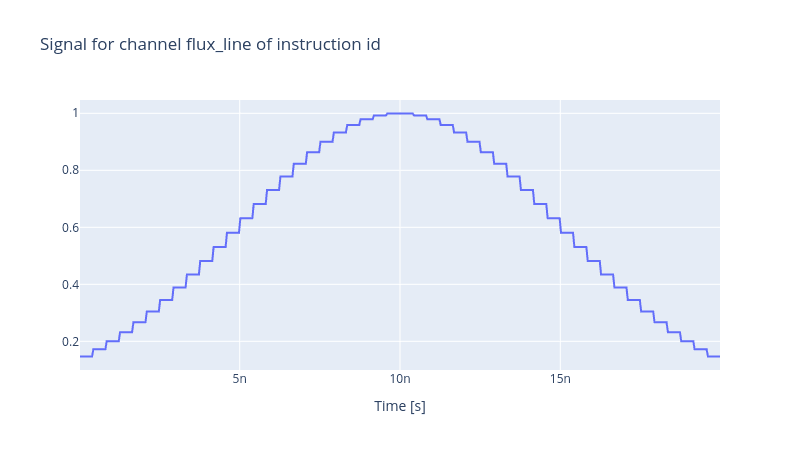
For a more appealing visualisation of the effect of the DAC component, let us define a Gaussian envelope so that the discretisation of the pulse is easily perceivable.

from qruise.toolset.signal import pulse

t_gate = stack_devices["AWG"].sim_time
gauss_params = {
    "amp": Qt(
        value=1.0, min_val=-2.5, max_val=2.5, unit="V"
    ),  # maximum amplitude of the Gaussian envelope
    "t_final": Qt(
        value=t_gate, unit="s"
    ),  # the final time at which the envelope is set to zero
    "sigma": Qt(value=0.25 * t_gate, unit="s"),  # the variance of the Gaussian envelope
}
gauss_env = pulse.Envelope(
    name="gauss_env",
    params=gauss_params,
    shape=pulse.envelopes.gaussian_nonorm,  # here we specify the shape of the envelope
)

And assign an identity instruction to the envelope.

from qruise.toolset.signal import gates
from qruise.toolset.libraries import constants

instr = gates.Instruction(
    name="id",  # name of the instruction
    t_end=t_gate,  # duration of the instruction (pulse duration)
    channels=["flux_line"],  # to which channel the instruction (pulse) is applied
    targets=[0],  # the index of the target qubit (not relevant but mandatory)
    ideal=constants.Id,
)

instr.add_component(comp=gauss_env, chan="flux_line")

We can now declare the Generator to produce the output pulse. Note that if we set the resolution of the Generator at low values, the step-like profile of the signal, due to the DAC component, may not be visible. We can set the resolution to a higher value to resolve those fine details.

from qruise.toolset.generator.generator import Generator

generator = Generator(devices=stack_devices, chains=stack_chain)
generator.draw(instr=instr, resolution=10 * stack_devices["AWG"].samp_rate)