The most minimalistic control stack is the one with solely an arbitrary waveform generator (AWG). It is one of the indispensable elements of a control stack as it enables one to have precise control over the shape and amplitude of the desired output pulse. One such setup is when a flux line goes to a superconducting target qubit, and one aims to tune the qubit frequency. Hence no local oscillator is involved. To model such a control stack, one needs to define a few things, the first of which is a flux (drive) line.

from qruise.toolset.libraries import components, hamiltonians

drive_line = components.Drive(
    name="flux_line",
    connected=["Qubit_0"],
    hamiltonian_func=hamiltonians.z_drive,
)

Since, for the time being, we are only examining the behaviour of the control stack, the name of the qubit is irrelevant, and for simplicity, we called it Qubit_0. The coupling between the control stack and the qubit via the flux line is via the z-axis component.

Then proceed with defining the control stack connected to this flux line, and let us start with defining our AWG. The Qruise toolset models a fistful set of parameters of a generic AWG device; for instance, the sampling rate, minimum waveform length, waveform granularity, etc. In addition to these static parameters, some other features are dynamic characteristics of an AWG. Amongst them are the rise time, overshoot, ringing or converting the synthetically generated digitised pulse to an analogue signal. These are modelled as pseudo-devices in the Qruise toolset, and we encourage the reader to refer to other blog posts dedicated to these pseudo-devices.

from qruise.toolset.objects import Quantity as Qt
from qruise.toolset.generator.devices import OEMAWG, VoltsToHertz

# simulation resolution, different than the AWG sampling rate
sim_res = 1e11

# dictionary of AWG parameters
awg_params = {
    "name": "AWG",  # given name of the device
    "sim_time": 20e-9,  # 20ns (pulse duration)
    "samp_rate": int(2.4e9),  # 2.4 GHz sample rate
    "waveform_granularity": 8,  # granularity of the AWG device
    "min_waveform_len": 16,  # shortest (in number of samples) waveform AWG can produce
}

# devices in the control stack
stack_devices = {
    "AWG": OEMAWG(**awg_params),
    "V2Hz": VoltsToHertz(
        name="V2Hz", V_to_Hz=Qt(value=1.0, unit="V/Hz")
    ),  # see the note below
}

# connectivity between different components of the control stack
# i.e. AWG (Source) -> V2Hz -> Pulse (Output)
stack_chain = {"drive_line": {"AWG": [], "V2Hz": ["AWG"]}}

The total duration of the waveform multiplied by the sampling rate of the device yields the total number of sample points of the final waveform that must satisfy two conditions (i) must be divisible by the granularity of the device, in this case, 8, and (ii) must be greater or equal to 16 which is the smallest number of samples the AWG can produce. Here, the AWG sample rate is 2.4GHz, and the intention is to generate a pulse with a 20ns duration. Hence there are in total 2.4e9 * 20e-9=48 sample points, a number which is divisible by 8 and is greater than the smallest number of sample points 16.

For our AWG to produce a signal, one needs to define two more entities; an Envelope and an Instruction. Whilst the former specifies the signal shape, the latter is a gate instruction. It is an abstraction layer that encapsulates the information of the envelope and the carrier of a pulse. Let us assume the Gaussian envelope.

from qruise.toolset.signal import pulse

t_gate = stack_devices["AWG"].sim_time
gauss_params = {
    "amp": Qt(
        value=1.0, min_val=-2.5, max_val=2.5, unit="V"
    ),  # maximum amplitude of the Gaussian envelope
    "t_final": Qt(
        value=t_gate, unit="s"
    ),  # the final time at which the envelope is set to zero
    "sigma": Qt(value=0.25 * t_gate, unit="s"),  # the variance of the Gaussian envelope
}
gauss_env = pulse.Envelope(
    name="gauss_env",
    params=gauss_params,
    shape=pulse.envelopes.gaussian_nonorm,  # here we specify the shape of the envelope
)

One may notice that the pulse amplitude is set at the Envelope level and is not a parameter of the AWG device. Finally, let us declare the Instruction object. Since we are not going to apply any gate operation on the target qubit, the simplest instruction one can think of would be an identity operation.

from qruise.toolset.signal import gates
from qruise.toolset.libraries import constants

instr = gates.Instruction(
    name="id",  # name of the instruction
    t_end=t_gate,  # duration of the instruction (pulse duration)
    channels=["drive_line"],  # to which channel the instruction (pulse) is applied
    targets=[0],  # the index of the target qubit (not relevant but mandatory)
    ideal=constants.Id,
)

# add the envelope to the instruction
instr.add_component(comp=gauss_env, chan="drive_line")

Finally, we need a Generator to generate the Gaussian pulse, hence the name. The Generator receives the list of devices and their interconnectivity.

from qruise.toolset.generator.generator import Generator

generator = Generator(devices=stack_devices, chains=stack_chain)
generator.draw(instr=instr, resolution=stack_devices["AWG"].samp_rate)

---

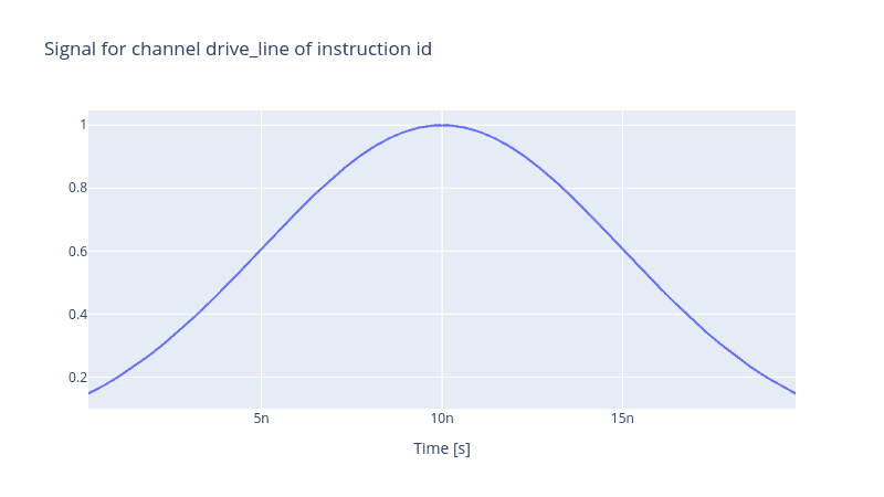
Note: VoltsToHertz is not an actual device. Its sole purpose is to convert the voltage to Hertz and is chip specific. For the purpose of demonstration here, the scaling is set to 1 V/Hz to have it act as a unit element.