We’re excited to introduce a new version of the qruise-toolset! This flexible software library is carefully designed to simulate and optimise quantum systems in a way that allows for easy customisation and smooth calculations. The latest updates to the qruise-toolset library, which is included in our advanced model learning software QruiseML, provide a new way of organising and understanding the most important concepts, providing users with a more streamlined experience.

What should users expect to gain from this update?

• A logical interface that reuses code, allowing users to easily set up new simulations and optimisations

• Seamless integration with QuTiP

• A modular design that reduces interdependency and gives the user the freedom to write minimal code

• Faster prototyping and feature releases with improved code quality and maintainability

• Improved performance and efficiency, minimising resource utilisation

• A library designed for parallel execution and seamless gradient-based optimisation

• Improved documentation with many example use-cases for various quantum computing hardware platforms

What are the new features?

Hamiltonian description

The Hamiltonian is defined in two parts:

• The stationary Hamiltonian is created using the Hamiltonian class

• The time-dependent Hamiltonian is added separately using the add_term() function, where the first input specifies time-independent pre-factors (e.g., operators and stationary parameters) and the second input specifies the time-dependent term (e.g., the drive).

# define stationary Hamiltonian
H = Hamiltonian(sigmaz())

# define time-dependent Hamiltonian
H.add_term(sigmax(), drive)

Quantum simulation problem

The Problem() class is used to specify a quantum simulation problem and is instantiated with the equations and parameters that govern the system:

• the Hamiltonian, H

• the initial condition (state vector or density matrix), y0

• parameters that uniquely parametrise the Hamiltonian, params

• the time interval of the simulation, (t0, t1)

The user chooses which equation they want the Problem to solve; for example, the Schrödinger equation or a master equation.

# define initial condition
y0 = np.array([1.0, 0.0], dtype=jnp.complex128)

# instantiate Problem with required inputs
prob = Problem(H, y0, params, (t0, t1))

# Solve Problem
prob.schroedinger()     # using Schroedinger equation
prob.von_neumann()      # using von Neumann equation
prob.lindblad(c_ops)    # using Lindblad master equation

Solvers

The qruise-toolset provides two pre-built solvers for computing system dynamics:

• Ordinary differential equation solver, ODESolver : uses diffrax for numerical integration, allowing flexibility in solver choice (e.g. diffrax.Tsit5()) and parameters, such as tolerances (atol,rtol) and step size (dt0)

• Piece-wise constant solver, PWCSolver : used when ODE solvers fail to converge; requires discretisation of the time domain with a fixed time step

# Option 1: ODESolver
solver = ODESolver(
diffrax.Tsit5(),
dt0=None,
saveat={"ts": ts},
atol=1e-8,
rtol=1e-6
)

# Option 2: PWCSolver
solver = PWCSolver(dt=1e-10, store=True)

# solve Schroedinger equation using PWCsolver
solver.set_system(prob.schroedinger())

Quantum optimal control problem

Similar to the quantum simulation problem, the qruise-toolset also includes a quantum optimal control problem, QOCProblem. In addition to the required inputs for Problem, QOCProblem also requires a target state, yt, and a loss function, loss. The loss function specifies the aspect of the system's performance that needs to be minimised to achieve optimisation, such as the infidelity.

# define target state
yt = np.array([0.0, 1.0], dtype=jnp.complex128)

# instantiate quantum optimal control problem with required inputs
opt_prob = QOCProblem(H, y0, params, (t0, t1), yt, loss)

Ensemble problem

An EnsembleProblem can be used to parallelise a simulation over an ensemble of parameters, initial conditions, or time spans. There are two flavours of EnsembleProblem:

• Element-wise product: the size of parameters, initial conditions, and time spans must match

• Cartesian product: the size of parameters, initial conditions, and time spans can be chosen arbitrarily. The resultant ensemble is the Cartesian product (different combination) of different initial conditions, parameters, and time spans.

# define parameters with multiple values for "a"
params = {
"a": jnp.linspace(1.0e7, 1.0e8, 50),
"w": 0.8 * t1,
"omega": jnp.pi / t1 / 2
}

# solve EnsembleProblem parallelised over “a”
prob = EnsembleProblem(H, (y0, None), params, (t0, t1))

Signal chain

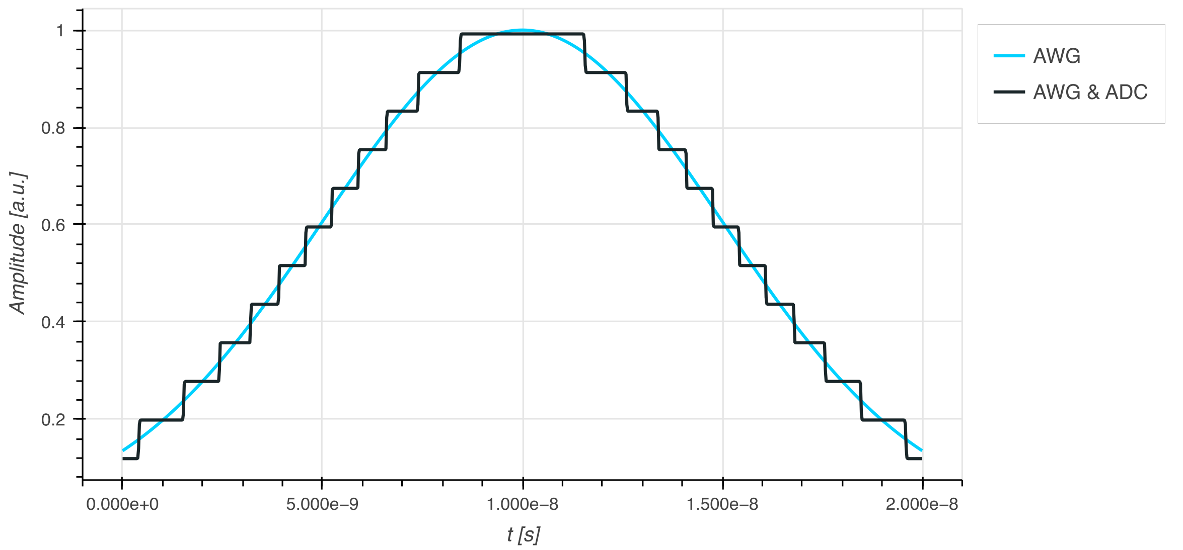
To easily emulate the behaviour of a control stack, a signal chain can be created where each component is added to the chain as a device or pseudo-device. This allows the user to model the impurities in signal generation, tune parameters to optimise gate operations, and counteract unwanted effects by designing suitable filter functions.

# store Gaussian parameters in dictionary
gauss_params = {
"amplitude": (amplitude, True),
"mean": (mean, True),
"sigma": (sigma, True),
}

# store ADC parameters in dictionary
adc_params = {
"nob": (nob, True),
"min_range": (min_range, True),
"max_range": (max_range, True),
}

gauss = Gaussian()
adc = ADC()
signal = Signal("ADCSimulation")

# add Gaussian and ADC as components named "AWG" and "ADC"
signal.add_from(["AWG", "ADC"], [gauss(), adc()], [gauss_params, adc_params])

Parameter collection

The ParameterCollection class provides a centralised and structured way to manage parameters, ensuring a single source of truth while avoiding inconsistencies or dangling definitions. It supports validation, batch updates, individual modifications, and clear representations, making parameter management reliable, efficient, and extendable.

pc = ParameterCollection()

params = {"amp": 1.0, "sigma": 2.0}
pc.add_param("key", 1.0)    # add parameter to parameter collection
pc.add_dict(params)         # add set of parameters
pc.get_val("key")           # get value of parameter "key"
pc.get_collection()         # gets all parameters in collection

Documentation website

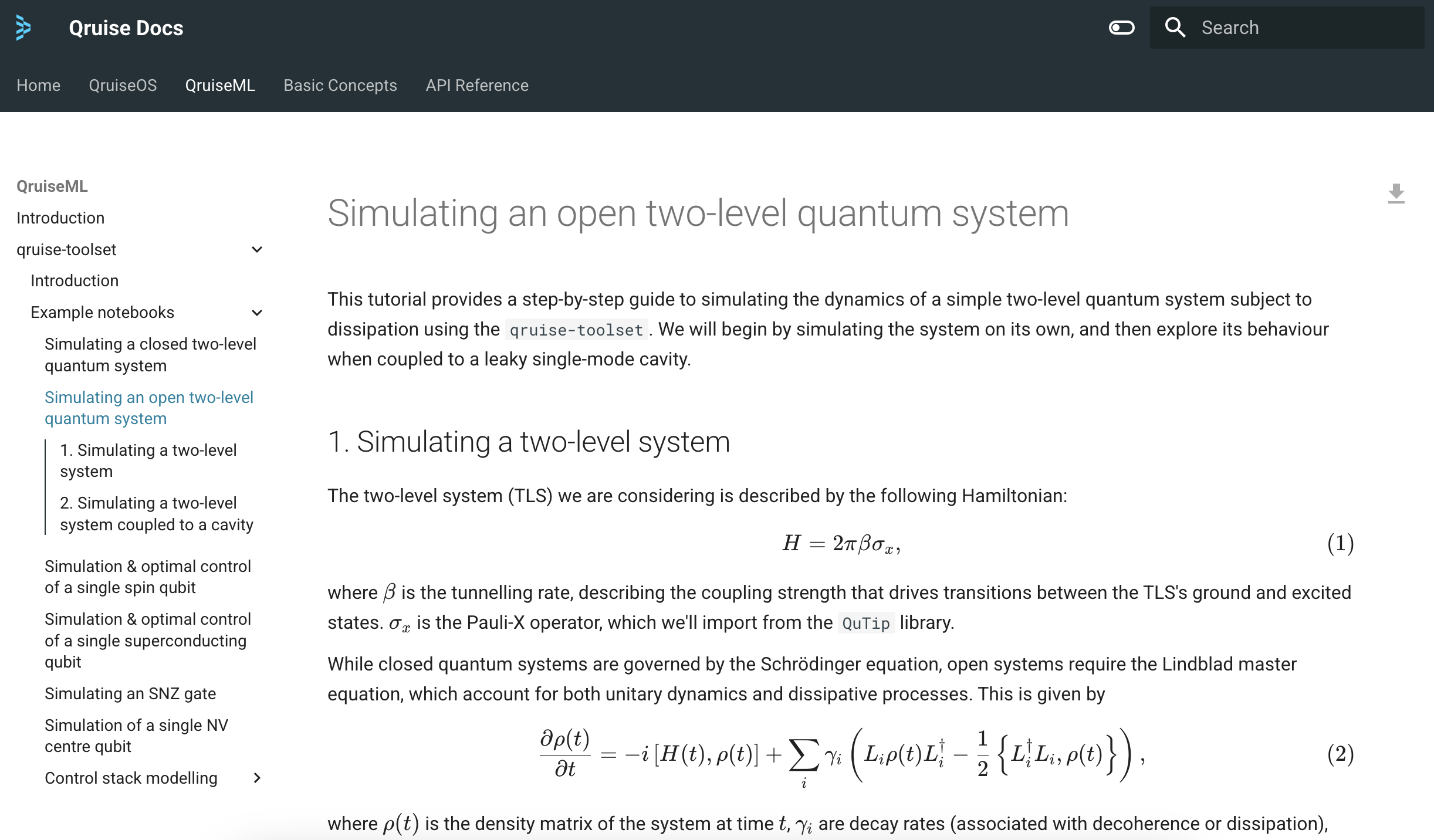
We've also launched a fully revamped documentation website for the qruise-toolset at docs.qruise.com/qruiseml/toolset/intro. This features walk-through examples at varying levels of complexity for many different quantum technology platforms, starting from simple two-level systems, and building up to sophisticated control stack modelling. These examples are available as executable Jupyter notebooks, making it easy to get started with the qruise-toolset.

More updates coming soon!

Stay tuned for more updates, including additional features for noise modelling and performance benchmarks to compare the qruise-toolset with other tools in the quantum field!

Contact us today at info@qruise.com to get access to the qruise-toolset or book a demo now!