In this blog post, designed to accompany our second introductory video, we're going to go over the second of our introductory notebooks, showing you how to set up both Calibration and Model Learning with the Qruise toolset. If you're interested in learning about setting up a device, and working on optimal control then our other blog post goes through that in a lot of detail.

Try it Yourself

If you're interested in running this tutorial or trying one of our examples of preconfigured devices (superconducting/Rydberg/ion trap/etc) on our demo JupyterHub, fill out our form or email us at demo@qruise.com and we'll get you set up.

Table of Contents

• Introduction
• Calibration
• Model Learning

Introduction

We're going to start by assuming you've followed the model setup in the previous tutorial notebook. This explains some of the key concepts inside Qruise and how to define the model that we're going to work with here.

If you still want to follow along with this tutorial you can use the create_experiment function inside single_qubit_experiment to get an example up and running quickly.

Calibration

The process of calibrating your quantum device involves gradient-free tuning of the experimental parameters within the experiment. This can be incredibly time consuming, and pretty fiddly to get right. Qruise simplifies this with its Calibration class that encapsulates all of the important information for doing calibration.

In this example we'll be using an ORBIT procedure which is a clever way to estimate gate fidelity. We will define some sequence of gates that when applied one after another result in an identity gate if all the gates are perfect. If they're not (which is typically the case) then we can measure the deviation from the identity gate to get an estimate of the imperfections in our system.

from qruise.toolset.utils import qt_utils
qt_utils.single_length_RB(RB_number=1, RB_length=5, target=0)

This code generates a sequence (in this case actually just 1 set) of gates for randomized benchmarking, where each sequence will consist of 5 gates where we target the 0 state of the qubit.

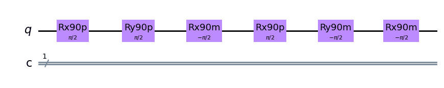
It's also possible inside Qruise to use Qiskit to visualise the sequences that we've generated We start by importing all the necessary modules:

from qruise.toolset.qiskit.gates import RX90pGate, RX90mGate, RY90pGate, RY90mGate
from qiskit import QuantumCircuit
from typing import List

then we use the Qiskit code to plot the random sequence that we generated:

QISKIT_GATE_MAP = {
    "rx90p": RX90pGate,
    "rx90m": RX90mGate,
    "ry90p": RY90pGate,
    "ry90m": RY90mGate,
}


seqs = qt_utils.single_length_RB(RB_number=3, RB_length=2, target=0)

circuits = seqs_to_circuit(seqs)

The next step is to communicate with your hardware, in the notebook we use simulated hardware but it's pretty easy to tweak this to work with any hardware you've got in your lab. Once again we start with some imports:

import numpy as np
import tensorflow as tf
from qruise.qiskit import create_provider, GenerateSvg

### ORBIT meta-parameters ###
RB_length = 25  # How long each sequence is in number of gates
RB_number = 10  # How many sequences
shots = 1000  # How many averages per readout

Then we can create a Qruise simulator of the physics to work out everything else that we need to do for the calibration:

orbit_provider = create_provider()
orbit_backend = orbit_provider.get_backend("qruise_qasm_physics_simulator")
orbit_exp = blackbox

then we define the fidelity function which will generate a sequence, simulate it, and then return the mean of the populations:

def ORBIT_qiskit_fidelity(params):

    populations = []
    results = []
    results_std = []
    shots_nums = []

    # Creating the RB sequences
    seqs = qt_utils.single_length_RB(RB_number=RB_number, RB_length=RB_length, target=0)
    orbit_exp.set_opt_gates_seq(seqs)  # speeds up the simulation of circuits
    circuits = seqs_to_circuit(seqs)
    orbit_exp.set_parameters(params, gateset_opt_map)

    # generate SVG only for a first circuit
    orbit_job = orbit_backend.run(
        circuits, exp=orbit_exp.asdict(), svg=GenerateSvg.FIRST
    )
    populations = [
        list(result.data.state_pops.values()) for result in orbit_job.result().results
    ]

    for pop in populations:
        excited_pop = np.array(pop[1:]).sum()  # total excited states population
        results.append(np.array([excited_pop]))
        results_std.append([0])
        shots_nums.append([shots])

    goal = np.mean(
        results
    )  # average of the excited state populations from every circuit
    return goal, results, results_std, seqs, shots_nums

Qruise has a really simple interface for calibration, which is shown below. Qruise gives you some parameters as a vector, and you map those to your scalar fidelity. You can also optionally return some stats about the calibration run, results, results_std, seqs, shots_nums if you want, but its not required. If you're not returning them then you can leave them blank We've also seen a lot of success by calibrating setting up a simple REST API on a server and using the requests library in Python. You can then define a fidelity function like so:

import requests
def get_fidelity_from_server(params, url="http://127.0.0.1:8080/..."):
    resp = requests.post(url, json={"params": params})
    return resp.json(), None, None, None, None

this makes it easy to interface with an existing experiment, just set up a server on you experiment computer and send the requests! At this point we're ready to set up our calibration step, we import the optimizer object and the desired algorithms:

from qruise.toolset.libraries.algorithms import cmaes
from qruise.toolset.optimizers.calibration import Calibration

We're going to use CMA-Es here, but we can wrap any algorithms that come from SciPy so if there's something missing then let us know! We can define a dictionary of options that we are going to pass to the optimizer

alg_options = {
    "popsize": 10,
    "maxfevals": 100,
    "init_point": "True",
    "tolfun": 0.01,
    "spread": 0.1,
}

and then we can capture all of that relevant information inside the Calibration object:

from qruise.toolset.optimizers.loggers import PlotLogger, PlotBestPointChart

log_dir = "logs/full_loop_calibration"

opt = Calibration(
    dir_path=log_dir,
    run_name="ORBIT_cal",
    eval_func=ORBIT_qiskit,
    pmap=parameter_map,
    algorithm=cmaes,
    options=alg_options,
    logger=[
        PlotBestPointChart(
            batch_size=alg_options["popsize"],
            xlim=alg_options["maxfevals"] / alg_options["popsize"],
            init_point=True,
        )
    ],
)

and then we're ready to run the calibration and see what we get!

opt.optimize_controls()

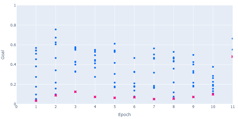
You can see here each of the epochs of the algorithm, where the blue points are the different sets of parameters that were evaluated and the red point is the best result from each epoch. You can see the general trend of improvement in the figure of merit.

Model Learning

Now calibrating your experiment is all well and good, you've improved some figure of merit that you're measuring but you still want to improve the model with the data you've collected! Optimal control is typically much faster when you do it on an accurate model of the system. We can use model learning to improve the accuracy of our model by finding parameters that more accurately match our data than what we were using before. This can feel a bit like a superpower once you get used to it, and it allows us to make use of all the experimental data that you've collected. We start by loading in the data

DATAFILE_PATH = os.path.join(log_dir, "recent/dataset.pickle")

with open(DATAFILE_PATH, "rb+") as file:
    data = pickle.load(file)

if you're looking to load your own data then we've got some helpful helper util functions that can prepare it into the correct format for use quickly We then need to set up our model learning object, since we're going to be learning a Qruise model we need to set one up, in this example notebook we're using the model from our previous blog post, so the hard part is already done for us. If you're developing a model for use inside Qruise for simulation, the same model can be used here Again we specify the opt_map of parameters that we'd like to optimise, in this case we're going to learn more accurate values for them

exp_opt_map = [[("Q1", "anhar")], [("Q1", "freq")]]
parameter_map.set_opt_map(exp_opt_map)

In this case we want to learn the frequency and anharmonicity of qubit 1. We then set up the model learning part of the code, this bit is pretty complex as you can probably imagine. There are also a whole load of parameters that you can tweak, and we can also combine algorithms together if we want both the benefits of gradient based and gradient free approaches

datafiles = {"orbit": DATAFILE_PATH}  # path to the dataset
run_name = "simple_model_learning"  # name of the optimization run
dir_path = "ml_logs"  # path to save the learning logs
algorithm = "cma_pre_lbfgs"  # algorithm for learning
# this first does a grad-free CMA-ES and then a gradient based LBFGS
options = {
    "cmaes": {
        "popsize": 12,
        "init_point": "True",
        "maxfevals": 150,
        "stop_at_convergence": 10,
        "ftarget": 4,
        "spread": 0.05,
        "stop_at_sigma": 0.01,
    },
    "lbfgs": {"maxfun": 50, "disp": 0},
}
sampling = "high_std"  # how data points are chosen from the total dataset
batch_sizes = {"orbit": 2}  # how many data points are chosen for learning
state_labels = {
    "orbit": [
        [
            1,
        ],
        [
            2,
        ],
    ]
}

Now we capture all of the relevant options and data inside the ModelLearning object and we pass the simulation that we want it to use into it

opt = ModelLearning(
    datafiles=datafiles,
    run_name=run_name,
    dir_path=dir_path,
    algorithm=algorithm,
    options=options,
    sampling=sampling,
    batch_sizes=batch_sizes,
    state_labels=state_labels,
    pmap=parameter_map,
    logger=[PlotLineChart()],
)

opt.set_exp(simulation)

Our next step is the most complicated and hardest to excute:

opt.run()

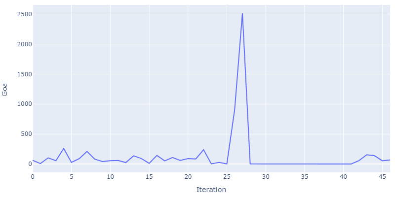
You can see here the progress of the model learning, there's a big jump as the algorithm hops out of a local minima and continues to optimize the parameters.

We can see how the model learning learns the anharmonicity of the qubit:

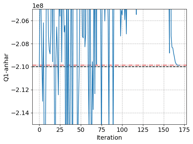
And how it learns the frequency of the qubit accurately:

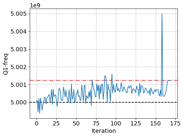
And there, we've done it... This step can take quite a long time, its one of the most complicated and it will often need quite a lot of steps before it converges to something satisfactory. The final step, and this will be specific to your problem, is this visualisation of your results from the model learning, in this case since we're showing an example problem we know what the actual values that we are looking for are and we can make some nice looking plots of how close we got with model learning.