While superconducting qubits definitely still dominate the main research interests of the big quantum computing companies there has of late been a good deal of interest in Rydberg atoms systems. These highly excited states of Cs or Sr atoms offer an exciting testbed for quantum computing and sensing applications. By placing the atoms using optical tweezers it is possible to create a "lattice" of atoms in almost an arbitrary configuration. These can then be addressed using globally applied pulses to perform gates.

In this blog post

• The system
• The simulation
• Optimising the pulses
• Optimal control

In this blog post we're going to show a short demonstration of how to use the Qruise toolset to Rydberg atoms into an anti-ferromagnetic state. We'll show one example, using the Qruise toolset to model and simulate a Rydberg system, using an initial guess pulse we can get a pretty good guess at the right but it's not perfect. To improve this we can use the Qruise toolset to optimize a pulse where the target state is an AFM state (we'll use the Neel structure factor as our goal). This let's us produce a close to perfect AFM state with pulses that are likely experimentally viable.

The work in this notebook is based on Vincent Lienhard's paper, Observing the Space- and Time-Dependent Growth of Correlations in Dynamically Tuned Synthetic Ising Models with Antiferromagnetic Interactions, where arrays of Rydberg atoms were programmed and whose correlations were studied.

The system

The Hamiltonian for a two atom system is:

$H/\hbar=\frac{\Omega(t)}{2} \sum*{i} \sigma*{i}^{x}-\frac{\delta(t)}{2} \sum*{i} \sigma*{i}^{z}+\sum*{i<j} U*{i j} n*{i} n*{j}$

where:

• $\hat{n}_{i} = (1 + \sigma_{z}) / {2}$
• $U = u_{pot}/ R_{ij}^{-6}$ with $R_{ij}$ the distance between the two atoms
• $\Omega(t)$ and $\delta(t)$ are time dependent pulses

We start by defining the relevant parameters for the system. We'll use the following values:

Omega_max = 2.3 * 2 * np.pi  # MHz
U = Omega_max / 2.3  # MHz
delta_0 = -6 * U
delta_f = 2 * U
blockade_radius = (5420158.53 / U) ** (1 / 6)

Our initial guess sweep pulse will be defined as follows:

t_rise = 252e-9
t_fall = 500e-9
t_sweep = (delta_f - delta_0) / (2 * np.pi * 10) * 10 ** (-6)
t_final = t_rise + t_fall + t_sweep

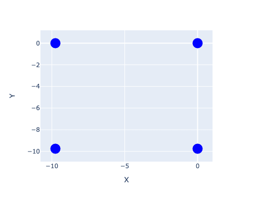
Rydberg atoms sit in a lattice, in Qruise we can create a lot of different shapes of lattice, or simply load one as a list of coordinates. In this case we will include a 2D square lattice with 2 atoms on each side:

n_side: int = 2
lattice = SquareLattice(n_side=n_side, r_interatomic=blockade_radius)
qubit_position_list = lattice.get_component_positions()
lattice.draw()

The simulation

The next step in simulating a Rydberg atom system is to define the RydbergSystem in Qruise. This captures all of the relevant information about the atoms and their interactions. It also allows us easily to simulate their dynamics:

ryd_system = RydbergSystem(lattice=lattice)

Next we need to add some drives, a quantum system without drives isn't particularly interesting. In this case we'll add two global drives to the system, these are an amplitude and detuning drive. The helper functions of the RydbergSystem class make this easy:

rydberg_name_list = [ryd.name for ryd in ryd_system.rydberg_atom_list]
ryd_system.add_drive("amplitude", "amplitude_afm", connected=rydberg_name_list)
ryd_system.add_drive("detuning", "detuning_afm", connected=rydberg_name_list)

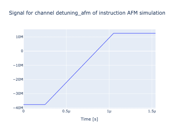
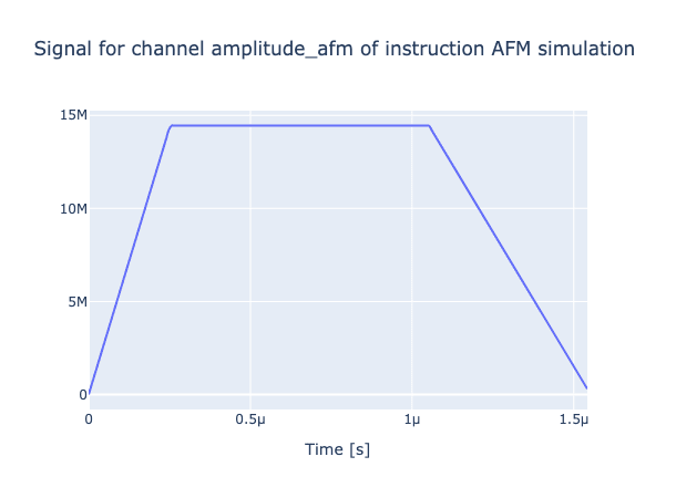
We want to give a good initial guess to the algorithm, so we can use a scalene trapezoid amplitude pulse and a linear ramp detuning pulse. We start by defining the parameters of these pulses:

scalene_trapezoid_amplitude_params = {
    "amp": Quantity(value=Omega_max, min_val=-0.1, max_val=300.0, unit="V"),
    "slope_factor": Quantity(value=1.0),
    "rise": Quantity(value=t_rise),
    "fall": Quantity(value=t_fall),
    "t_final": Quantity(
        value=t_final, min_val=0.9 * t_final, max_val=1.1 * t_final, unit="s"
    ),
}
linear_ramp_detuning_params = {
    "amp": Quantity(value=1.0, min_val=-100.0, max_val=100.0, unit="V"),
    "initial_amplitude": Quantity(value=delta_0),
    "final_amplitude": Quantity(value=delta_f),
    "rise": Quantity(value=t_rise),
    "fall": Quantity(value=t_fall),
    "t_final": Quantity(
        value=t_final, min_val=0.9 * t_final, max_val=1.1 * t_final, unit="s"
    ),
}

Next we create the pulse envelopes for the pulses. These essentially define the shape of the pulses, using the parameters that we just defined, while also giving a human readable description and name:

scalene_trapezoid_amplitude = pulse.Envelope(
    name="amplitude",
    desc="Scalene trapezoid envelope for amplitude",
    params=scalene_trapezoid_amplitude_params,
    shape=envelopes["scalene_trapezoid"],
)
linear_ramp_detuning = pulse.Envelope(
    name="detuning",
    desc="Linear ramp envelope for detuning",
    params=linear_ramp_detuning_params,
    shape=envelopes["linear_ramp"],
)

The second last step before we simulate the dynamics is to create a signal generator. In an experiment this is typically some digital to analogue converter or arbitrary waveform generator. Since we're just interested in the dynamics we can use a SimpleGenerator:

v2Hz = 1e6
generator = SimpleGenerator(
    V_to_Hz=Quantity(value=v2Hz, min_val=0.9 * v2Hz, max_val=1.1 * v2Hz, unit="Hz/V")
)
ryd_system.set_generator(generator)

Now the final step before we can simulate the dynamics is to add an instruction telling Qruise how long it needs to play each pulse for, you can think of this a bit like using sequencing mode on an AWG:

afm_instr = gates.Instruction(
    name="AFM simulation",
    t_start=0.0,
    t_end=t_final,
    channels=["amplitude_afm", "detuning_afm"],
)
ryd_system.add_instruction(
    afm_instr,
    [scalene_trapezoid_amplitude, linear_ramp_detuning],
    ["amplitude_afm", "detuning_afm"],
)

If we want to see our pulses then it's really easy to visualise them:

generator.draw(afm_instr, resolution=ryd_system.sim_res, centered=False)

and we can now simulate the dynamics of the system:

ryd_system.create_model()
ryd_system.create_experiment()
ryd_system.experiment.set_prop_method("Tsit5")
result = ryd_system.run()

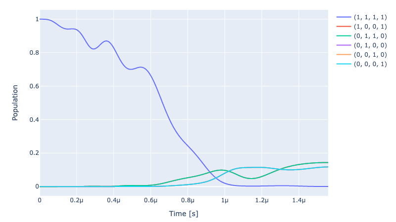
the propagators are computed and stored in the result object. They're also stored in the ryd_system too. We can now plot the dynamics of the system:

initial_state = ryd_system.get_initial_state()
sequence = [afm_instr.get_key()]
ryd_system.experiment.draw_dynamics(
    sequence, initial_state, best_scored=5
)

Optimising the pulses

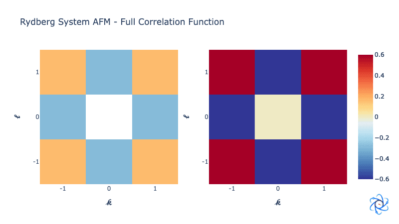
Previously we mentioned that we're going to use the Neel structure factor as the objective function. This deserves a bit of explanation. We can first define the spin-spin correlation function as: $g^{c}(k, l)=\frac{1}{N*{k, l}} \sum*{(i, j)=(k R, l R)}\left[\left\langle n_{i} n_{j}\right\rangle-\left\langle n_{i}\right\rangle\left\langle n_{j}\right\rangle\right]$

and then from this we can define the Neel structure factor: $S*{\text {Néel }}=4 \times \sum*{(k, l) \neq(0,0)}(-1)^{|k|+|l|} g^{c}(k, l)$ Basically we're going to use Qruise to try and optimize this function using a parameterised pulse.

For our initial guess we can plot the full correlation function of the states, on the right we can see the ideal full correlation function:

ryd_system.draw_full_correlation_function(show_pure_afm=True)

Optimal control

There are a whole load of techniques that you can use to do optimal control but most of them boil down to simplifying the problem to a form that you can more easily solve. In this example we will use a dCRAB like optimization. To perform this algorithm we expand our control in terms of a fourier series and search for the amplitudes of each of the fourier components. This simplifies the search problem drastically and is typically done with Nelder-Mead. However in Qruise we have access to a whole load of different optimizers, and since our model is fully differentiable, we can actually use gradient based search methods to find the optimal values (it's an approach that's really similar to GROUP).

We start by adding two new drives to the system, one for the amplitude and one for the detuning. We also add a new instruction to the system:

# Amplitude variation and frequency number
amplitude_variation: float = 2.0
freq_number: int = 20
freq_limits: list = [0.01, 3.0] # [0.01, 8.0]

opt_crab_amplitude = ryd_system_opt.create_CRAB_envelope(
    name="optimized_amplitude",
    t_final=t_final,
    ampl_var=amplitude_variation,
    freq_number=freq_number,
    initial_random_value=True,
    freq_limits=freq_limits,
)

opt_crab_detuning = ryd_system_opt.create_CRAB_envelope(
    name="optimized_detuning",
    t_final=t_final,
    ampl_var=amplitude_variation,
    freq_number=freq_number,
    initial_random_value=True,
    freq_limits=freq_limits,
)

# Create the instruction and associate it to the envelopes and drives
afm_opt_instr = gates.Instruction(
    name="AFM_optimization",
    t_start=0.0,
    t_end=t_final,
    channels=["amplitude_afm", "detuning_afm"],
)

ryd_system_opt.add_instruction(
    afm_opt_instr,
    [cosine_12_amplitude, linear_ramp_detuning, opt_crab_amplitude, opt_crab_detuning],
    ["amplitude_afm", "detuning_afm", "amplitude_afm", "detuning_afm"],
)

Then we have to set up the opt_map for the parameters that we want to optimize.

ryd_system_opt.set_crab_map(
    instruction=afm_opt_instr,
    pulses=["optimized_amplitude", "optimized_detuning"],
    channels=["amplitude_afm", "detuning_afm"],
)

Then we just have to capture the important parameters of the optimal control algorithm inside the OptimalControl class:

opt = OptimalControl(
    dir_path=log_dir,
    fid_func=neel_factor,
    pmap=ryd_system_opt.parameter_map,
    algorithm=algorithms.cma_pre_lbfgs,
    options={
        "cmaes": {
            "popsize": 50,
            "maxfevals": 200,
            "init_point": "True",
            "tolfun": 0.01,
            "spread": 0.5,
        },
        "lbfgs": {"maxfun": 100, "ftol": 1e-10, "gtol": 1e-10},
    },
    run_name="afm_rydberg_2x2_120it_cmaes",
    logger=[PlotLineChart(ylim=[0, 1.2])],
    fid_subspace=rydberg_name_list,
    fid_func_kwargs=fid_func_kwargs,
)

and finally we do the optimal control:

opt.set_exp(ryd_system_opt.experiment)
opt.optimize_controls()

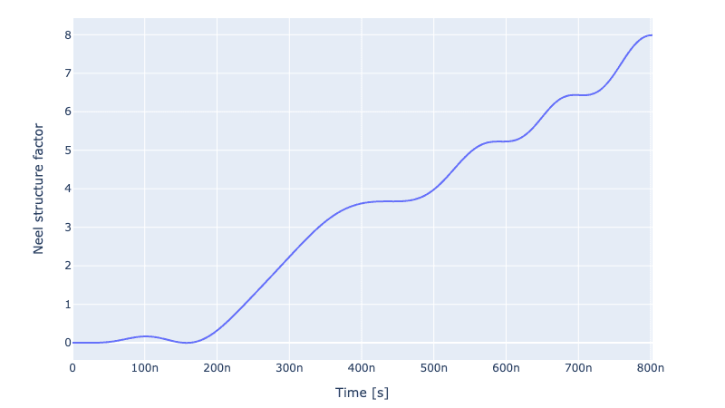
To verify that everything has worked we can plot the evolution of the Neel structure factor over time:

ryd_system_opt.draw_neel_dynamics(opt_sequence)

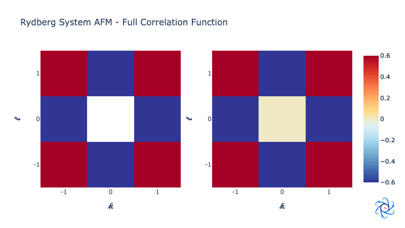
And we can plot the full correlation function of the states again:

ryd_system_opt.draw_full_correlation_function(show_pure_afm=True)